BISTRO: a general purpose oracle for macroeconomic time series

Predictions of macroeconomic variables are a key input to economic policy, yet traditional econometric approaches have the limitation that the model needs to be tailored to the specific task. The advent of large language models (LLMs) opens up the tantalising prospect that a single general model can tackle a wide variety of tasks. This article introduces the BIS Time-series Regression Oracle (BISTRO), a general purpose time series model for macroeconomic forecasting. Building on the transformer architecture underlying LLMs, BISTRO is fine-tuned on the large repository of macroeconomic data maintained at the BIS. We put the model through its paces by assessing how well it forecasts the 2021 inflation surge. In contrast to standard benchmarks, which mechanically project a reversion to the mean, BISTRO correctly anticipates the persistence of the inflation wave. This highlights its ability to adapt to unfamiliar patterns in the data. Thus, BISTRO holds promise for producing reliable baseline forecasts and for scenario analysis.¹

JEL classification: C32, C45, C55, C87

Predictions of macroeconomic aggregates are a key ingredient to economic policy, especially for monetary policymakers. Traditionally, forecasting has relied on time series models, where historical developments of key economic variables and their correlations are used to extrapolate the future path of the variable(s) of interest. In this traditional approach, each model is tailored to the specific task at hand, meaning it has to be constructed, estimated and validated for a single problem. When dealing with another task involving a different set of variables in another setting, another model designed specifically for the new problem needs to be built. To use an analogy, the modeller is like a carpenter who has access to a large box of diverse tools. A new task is tackled by figuring out how to use or modify tools that were created for another task.

The advent of large language models (LLMs) has popularised a very different approach to problem-solving. The latest generation of LLMs are like a Swiss army knife rather than a box of tools: they can tackle a wide range of problems, even ones that were unforeseen when the model was built and trained. In the industry jargon, LLMs are "zero-shot learners" or "foundational models".

The ever-growing capabilities of LLMs have opened up the tantalising prospect that a similarly flexible approach would support time series forecasting. Rather than having to build a bespoke model for a particular task, the same foundational model could be deployed for a wide variety of different tasks.² The main advantage of such a model is that forecasting can break free of the inflexibility of traditional econometric approaches, in which specific modelling choices must be imposed from the start.

This article introduces such a flexible model. We name it the BIS Time-series Regression Oracle (BISTRO). BISTRO builds on the machinery underlying LLMs and applies it to the world of economic time series.

The article starts with a general introduction to the mathematical principles underlying LLMs and explores why they have broader applicability beyond the domain of text. Just as LLMs do well in guessing the next word within the broader context of the sentences that precede it, foundational time series models do well in guessing the next realisation of a macroeconomic time series within the broader context of what else has been happening in the economy. The only difference is that they operate on macroeconomic variables rather than words. But mathematically, the task is identical.

We then demonstrate how BISTRO can assist economists in their forecasting and scenario analyses. For example, a researcher can produce a generic baseline forecast for, say, inflation and then evaluate how conditioning on different explanatory variables (and different assumptions for their evolution) modifies the baseline. Hence, BISTRO constitutes a low-cost and easy-to-use forecasting tool that performs well compared with traditional econometric benchmarks. In particular, we show how BISTRO anticipates the persistence and pervasiveness of the inflation surge in 2021.

BISTRO comes with detailed instructions and pre-compiled scripts on how to operate it, available at https://github.com/bis-med-it/bistro. To facilitate replication and practical use, these scripts can be run in Google Colab, allowing users to upload their own data set and generate baseline and conditional forecasts with BISTRO through a guided workflow.

From word prediction to foundational language models

Since the emergence of large language models (LLMs), economists have increasingly used them for text-based tasks such as drafting, coding and literature reviews.³ Artificial intelligence (AI) tools are now routinely applied across many areas of economic analysis and research.⁴

LLMs are valuable because they can handle a wide range of natural language processing (NLP) tasks without any modification to their structure or parameters. Models such as the Generative Pretrained Transformer (GPT) can translate text, summarise documents and write code – even though they were trained for a single and very specific task: predicting the next word in a sequence.⁵ This ability to perform tasks for which the model received no explicit training is known as zero-shot learning and is what makes LLMs foundational models: they are general purpose tools applicable to a broad set of tasks, possibly unforeseen when the model was created.

The zero-shot capability of transformers is rooted in how they represent words. In any quantitative model, words must first be converted into a vector of numbers, a process known as embedding. A simple approach would assign each word a fixed vector, regardless of context. But consider the word "bond": in isolation, it could refer to a financial instrument, a family connection or a fictional spy (BIS (2024)). A fixed, standalone vector cannot capture this range of use. Transformers address this limitation through contextualised embeddings. Rather than assigning a static vector to each word, the transformer reads the full surrounding text and constructs a vector that reflects the word's specific meaning in that specific context. The word "bond" would thus receive a different vector representation in a sentence about sovereign debt than in one about family relationships or spy fiction. This is achieved through the attention mechanism, a core component of the transformer architecture.⁶ Attention allows each word to attend to every other word in the input, weighting their contributions according to relevance. The result is a set of embeddings that encode not just the identity of each word, but its role and meaning within the input sequence.

As the model generates a different internal representation for every new input, it effectively adapts to the questions it is prompted with. This adaptation to the context is at the root of its flexibility. Within the given model, the context-dependent embeddings allow it to behave differently for each prompt. The term "foundational model" refers to such adaptability (a Swiss army knife as opposed to a box of different tools). It is this adaptability that distinguishes transformer-based LLMs from the older generation of expert systems and machine learning models.

From bespoke time series models to a general purpose forecasting tool

Traditional prediction and forecasting methods, whether rooted in econometrics or machine learning, share a common feature: each task calls for its own model. The researcher must first specify the model's functional form f and then estimate its parameters – typically a low-dimensional vector – using historical data. Then the forecasting equation from these traditional models can be written as:

where y is the target variable, and x and are, respectively, the data and the vector of estimated parameters on which the model depends, ie . The model functional form f(.;.) – be it a simple autoregressive model with one lag, such as an AR(1), a space-state model or even a random forest or a neural network – defines how the data included in the model specification are processed to produce parameter estimates and forecasts.

By contrast, a foundational model, such as BISTRO, takes a different approach. First, no functional form f is imposed on the data or the estimates derived from the data. Instead, it works with a very general function derived from the transformer model (see the Annex). Importantly, the foundational model takes as input not only the underlying data series x for the problem at hand but also parameters derived from other (potentially massive) data used in its training.

In the case of LLMs that work with text, their training set includes a substantial portion of text on the internet. Thus, when the LLM operates on a particular task involving a document, it employs data from outside for the specific task that it is asked to perform. In the case of BISTRO, the training set includes the large macroeconomic data set maintained by the BIS (see Box A). In this way, the predictive power of a foundational model derives from the training set of data that goes well beyond the data involved in a particular task.

More formally, we can contrast BISTRO with the traditional time series model by expressing the prediction as:

Here, the function g is the general predictive function derived from the transformer model (see the Annex for details). This takes as the inputs not only the data x for the specific problem at hand but also the vector which depends on a potentially vast set of other data Z that was used to train the model.

Note that both traditional econometric models and foundation models rely on the same information set, x, to predict future outcomes. The key difference lies in how they use this information. An econometric model operates in two steps: it first estimates the model parameters using x and then generates predictions conditional on the estimates . A foundational model, by contrast, operates in a single step: it maps x directly to predictions, relying entirely on weights, , that were estimated during pre-training and remain fixed at inference time.

The practical payoff for forecasters is considerable. With traditional methods, each change in the forecasting setup (eg adding a variable, lengthening the available sample, switching from a univariate to a multivariate model) calls for a new round of model-building and estimation. A foundational model subsumes all these cases. When provided with a single variable, it produces a non-linear autoregressive forecast in which the order is adapted automatically by the attention mechanism that decides which lags to include. If explanatory variables are included in the input, the model refines its predictions to reflect their influence – all without any change to the model's structure or parameters. Because the internal weights adapt to the data prompted, the model also naturally accommodates time-varying relationships.

Introducing the BIS Time-series Regression Oracle

Our BISTRO builds on the MOIRAI (Woo et al (2024)) architecture. MOIRAI is a prominent example of a foundational model for time series forecasting, adapting the transformer architecture from NLP to numerical sequences.⁷ Several features distinguish time series from text and require specific design choices. Words belong to a finite vocabulary; time series observations are realisations of continuous variables. Text follows a single reading order; time series can be sampled at different frequencies. Even more importantly, time series models may need to account for explanatory variables whose influence may change over time. MOIRAI addresses these challenges by grouping consecutive observations into fixed-length blocks (patches). A patch size of eight, for instance, means the model processes and predicts eight observations simultaneously. MOIRAI was trained on over 27 billion data points drawn from diverse domains (including energy, healthcare and economics/finance) with sampling intervals spanning one second to one year. It can incorporate up to 128 covariates, process variable patch sizes and handle multivariate time series.

While MOIRAI is a powerful general purpose tool, its broad training base means it is not optimised for any single application. As we will show below in the forecasting exercises, its predictive accuracy for macroeconomic variables is poor, particularly at longer time horizons or with covariates. We therefore constrained and fine-tuned MOIRAI to focus on macroeconomic time series and boost its usefulness for central banks, hence creating BISTRO.⁸

We made two main adjustments to build BISTRO. First, the model was limited to a daily frequency and a patch size of 32 days. This allows BISTRO to handle both unconditional forecasts – in which all variables are known only up to a given date – and conditional forecasts, in which some series are set to follow certain future paths. Second, the model was fine-tuned on the BIS macroeconomic data set (see Box A). All data were converted to a daily frequency by carrying forward the last known value until a new release or revision became available, ensuring that no future information entered the training process. The specific training procedure and model parameters are described in a companion working paper (Koyuncu et al (2026)).

BISTRO is therefore a foundational model tailored to macroeconomic time series typically observed at monthly or quarterly frequencies. It should not be regarded as the definitive answer to any forecasting or nowcasting exercise, but rather as a low-cost and easy-to-use tool that can quickly provide reasonable solutions to many forecasting and nowcasting problems. It can also serve as a benchmark: if a purpose-built econometric model cannot improve on BISTRO's predictions, it might call for additional model exploration. And, like any foundational model, BISTRO can be further fine-tuned, for instance to focus on a specific country or to address a particular forecasting problem.

How to operate BISTRO

BISTRO was designed as a ready-to-use and off-the-shelf tool for macroeconomic forecasting. This section describes the workflow, which comprises three stages: data preparation, parameter modelling, and forecasting and evaluation (Graph 1). A Google Colab notebook supports replication, with sample scripts and step-by-step code for the entire workflow, including rolling-window forecast generation.

In the data preparation step, the user aligns the target variable (eg inflation or unemployment) with selected covariates (eg oil prices or exchange rates) along the time dimension. Indicators released at different frequencies are converted to daily by carrying forward the last known value. This ensures that the data set contains only information available as of each date. For example, second quarter GDP appears in the data set only on its release date in the third quarter.⁹ The result is a (pseudo) real-time information set that mirrors the operational environment faced by central bank modellers and prevents forecasts from using data that were not yet available.

 

Graph 1

 

 Close all

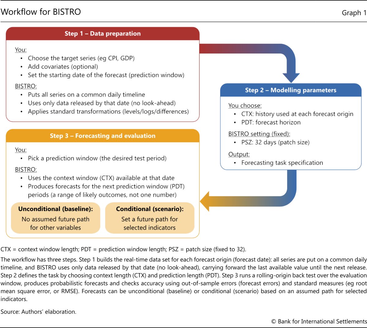
The aligned data set is then passed to the model interface, which automatically handles the required preprocessing. It applies standard data transformations (levels, logs, differences), imputes missing values due to publication lags and determines the number of past observations used for each prediction, based on the user-defined context window length (CTX). For instance, a context window of 100 patches corresponds to roughly 8.75 years of historical data. Users do not need to manually transform or reformat the data.

A simple example illustrates how running the model mirrors operational forecasting. Suppose the goal is to forecast inflation from 2023 through end-2025, estimating the next 12 months of inflation (12 patches of 32 days) at each forecast date, using 20 years of history (228 patches). BISTRO is first prompted with observations from 1 January 2003 through 31 December 2022 and then predicts inflation for the next 12 months. It then shifts the data window forward by one patch, using data from 1 February 2003 through 31 January 2023 to forecast the next 12 months. This process repeats until the end of the sample.

 

Graph 2

 

 Close all

BISTRO automates the entire estimation process and calculates prediction errors at each step. It benchmarks the results against an AR(1) model, enabling a quick assessment of forecast quality relative to a common benchmark. In the example, the user supplies consumer price index (CPI) inflation data for the country or area of interest over the period 2003–25, sets the CTX to 228 patches and the prediction window length (PDT) to 12 patches. The AR model is trained on data through December 2022 and is updated monthly, while BISTRO uses all 228 context patches at each forecast origin without retraining.

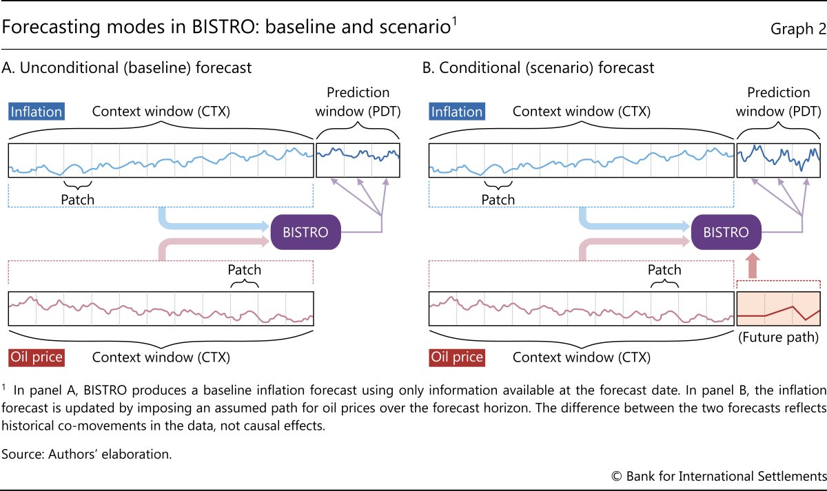
To produce forecasts that also depend on covariates such as oil prices or exchange rates, the user adds these series and aligns them with the target variable. BISTRO then conditions its prediction on both the past values of the target and the explanatory variables (Graph 2.A). BISTRO can also produce conditional forecasts. To this end, the user fixes the future path of one or more covariates and feeds them to the model (Graph 2.B). For example, BISTRO can forecast 2026 inflation under alternative oil price trajectories. This allows researchers to explore different macroeconomic scenarios in a straightforward way.

Forecasting inflation with BISTRO

This section illustrates how BISTRO can be used to forecast inflation. More specifically, we compare the results obtained by prompting BISTRO with historical inflation data against those obtained from a standard time series benchmark – namely a naive AR(1) – as well as against those produced by the baseline MOIRAI.¹⁰ We first examine the accuracy of BISTRO's unconditional forecasts – ie simple out-of-sample predictions that do not depend on covariates. Then we showcase how forecasts are affected by the inclusion of explanatory variables (covariates) and how they can be tweaked to reflect assumptions on the future evolution of said covariates. This is typically labelled a conditional forecasting exercise.

The unconditional forecasting exercise mimics a task of paramount relevance for central banks – predicting monthly inflation at short and medium horizons. To have BISTRO (and MOIRAI) generate unconditional forecasts, we prompt it with the past values of inflation, starting 240 months before the beginning of the forecast. Note that BISTRO relies on the same amount of information as provided for a benchmark AR(1) – that is the latest inflation readings. The AR(1) model uses 240 months of past inflation values to estimate its parameters and then applies exponentially decaying weights to the last observation to predict the next 12 months. In contrast, BISTRO directly predicts the next 12 months of inflation using the very same 240 months of data. Yet this does not require parameter estimation: BISTRO relies on pre-estimated parameters from its generic training process.

 

Graph 3

 

 Close all

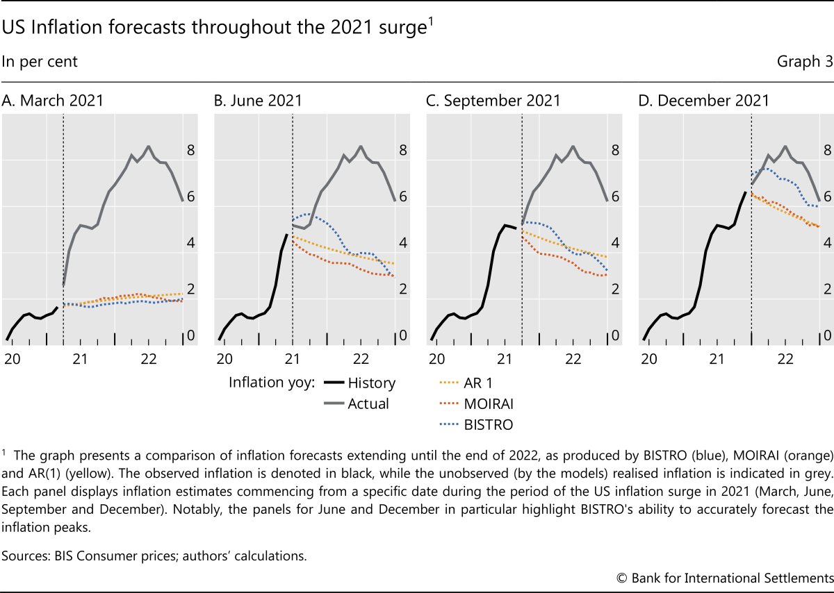
To illustrate BISTRO's forecasting capabilities, we first put it to test on the inflation wave of 2021–22.¹¹ Graph 3 shows US inflation forecasts made by BISTRO, MOIRAI and a benchmark AR(1) model, starting at different points of the inflation surge. Each panel shows multi-step-ahead forecasts, in which predictions are produced dynamically over the desired forecast horizon and hence do not rely on inflation readings that were not yet available. In March 2021, when inflation had not yet surfaced, all models provide a similar forecast of inflation converging towards the 2% target (Graph 3.A). Yet as the first signs of the inflation surge appear, in June 2021, the model projections diverge (Graph 3.B). The AR(1) benchmark mechanically decays towards the historical average, while the MOIRAI model hints at an even faster decline. By contrast, BISTRO correctly anticipates a more persistent wave of inflation. In September 2021 inflation had apparently plateaued, and while the AR(1) and MOIRAI stick to a declining trajectory, BISTRO hints at a shallower decline (Graph 3.C). In December, a second wave of inflation had already taken hold, and BISTRO foresees rising and persistently high inflation, close to the actual outcome (Graph 3.D).¹²

To be sure, the 2021–22 wave of inflation is a very specific episode which simple linear time series models have a hard time processing. The exercise above was indeed meant to illustrate how BISTRO can identify and deal with possible structural changes and regime shifts. Yet BISTRO performs competitively and consistently over different time periods, not necessarily featuring structural changes and extreme circumstances. To establish this, we run a full-fledged forecasting comparison based on four distinct evaluation windows: 1995, 2005, 2015 and 2023–24, which were not included in the BISTRO's training sample. These windows reflect markedly different macroeconomic regimes, ranging from the pre- and post-Great Financial Crisis period to the recent episode of elevated inflation.

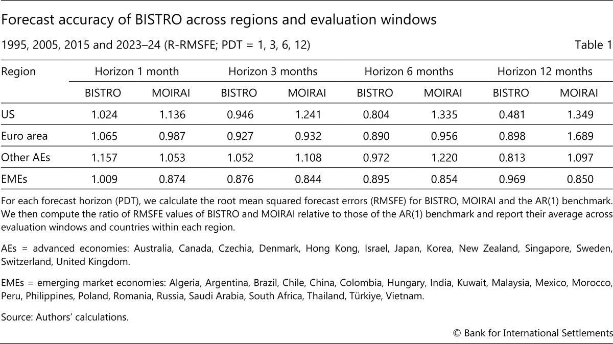
This forecasting setup allows us to assess model performance across phases characterised by different levels of volatility, sources of price pressures and potential structural changes. Within each evaluation window, we focus on forecasts of the year-on-year (yoy) growth in the CPI at one-, three-, six- and 12-month-ahead horizons (PDT = 1, 3, 6, 12). Forecasts are generated sequentially over the test window as it progresses forward in time.¹³ The analysis is conducted for all countries for which sufficient data are available. Forecasts are separate for each country, but for ease of presentation, results are aggregated into four groups: the United States (US), euro area, other advanced economies (other AEs) and emerging market economies (EMEs).¹⁴

The results show that BISTRO provides reliable and accurate forecasts compared with the benchmark. We measure forecast accuracy using relative root mean squared forecast errors (R-RMSFE) with respect to the AR(1) benchmark, averaged across countries and testing windows within each group (Table 1). So a value below one indicates that BISTRO (or MOIRAI) outperforms the benchmark. On average, BISTRO improves upon the benchmark in most cases, with particularly strong gains at the longer horizons. For the United States, BISTRO outperforms both AR(1) and MOIRAI for all horizons except the one-month-ahead, with its relative performance improving as the forecasting horizon lengthens. This is similar for the euro area, where both general purpose models perform similarly on average and improve with the length of the forecasting horizon. Results for other advanced economies are mixed, with average performance closer to the AR(1) benchmark.¹⁵ Similarly, for EMEs, BISTRO delivers systematic improvements at the medium-term horizon.

 

Table 1

 

 Close all

Constructing scenarios with BISTRO

Having established the solid performance of our model in unconditional forecasting, we turn to scenarios, that is, conditional modelling exercises. One of the main advantages of the flexibility of our model lies in its ability to naturally handle relevant covariates that one may want to condition the forecast on. In standard time series models, conditioning is possible only on the set of variables that were considered and explicitly included in the model's specification and estimation. We can instead prompt BISTRO with trajectories of additional macroeconomic variables (not necessarily featured in the training sample) and then generate projections that are conditional on their realisations. The way the model handles this is by relying on the historical patterns that emerge from the training data set and hence shape the embeddings.

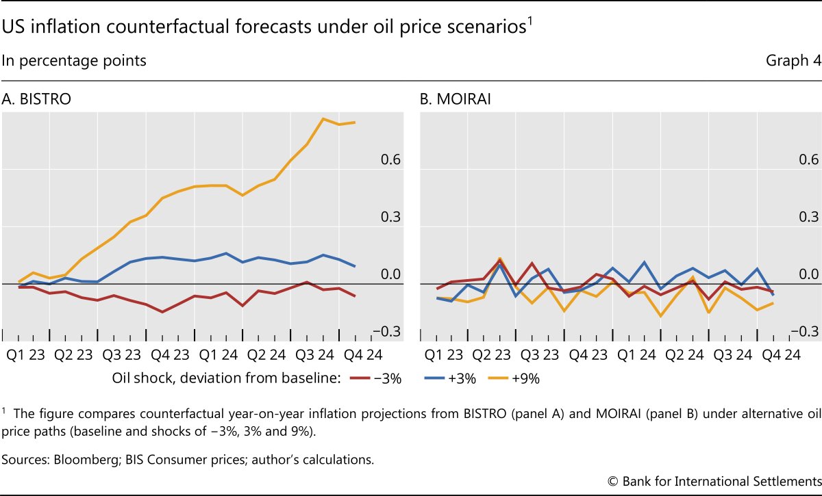
To illustrate this, we consider conditional forecasts of inflation based on different possible future trajectories of the oil price. Starting from its realised path, which serves as a baseline, we introduce counterfactual oil price scenarios in which the oil price would be 3% lower and 3% and 9% higher than it actually was. In general, conditioning on oil prices produces systematically higher or lower oil price paths relative to the baseline (Graph 4.A). But even more importantly, the model unveils a substantial degree of non-linearity in the reaction of inflation to oil prices. First, a decline in the price of oil has smaller medium-run effects on inflation than an increase by the same amount. Second, larger increases in the price of oil have a more than proportional effect on inflation. A clear bearing on the relationship between oil prices and inflation is one of the advantages of our model over MOIRAI. The latter, trained on a wider set of non-macroeconomic time series, fails to highlight any meaningful connection between oil prices and inflation (Graph 4.B).

 

Graph 4

 

 Close all

Monetary policy as viewed through the prism of BISTRO

While our model is a device to uncover (potentially non-linear and complex) correlations in the data, it relies entirely on the historical patterns that emerged during the training. Hence, it cannot provide insights into the effects on the observed time series of unobservable macroeconomic shocks, nor can it shed light on how structural forces with an economic interpretation contribute to its forecasts. So, for example, if one generated counterfactual scenarios based on different trajectories of monetary policy, one would see that higher policy rates are associated with higher inflation. This is because the model has no understanding of a policy rule or of how a "tighter" policy transmits to the real economy. Hence, conditioning on a policy rate trajectory will yield only a correlation based on historical patterns.

However, this suggests that the model can be used to gain insights on historical response functions, eg a Taylor rule for monetary policy. To do this, we turn to conditional forecasting exercises in which the model is provided with realised macroeconomic paths and asked to generate the implied policy rate projections based on such a macroeconomic outlook. More precisely, we condition the forecast for the US policy rate on the realised path of inflation and examine the implied trajectories of the policy rate obtained by providing different historical contexts. This design allows us to isolate how the historical information provided affects the model-embedded relationship between macroeconomic conditions and monetary policy.

 

Graph 5

 

 Close all

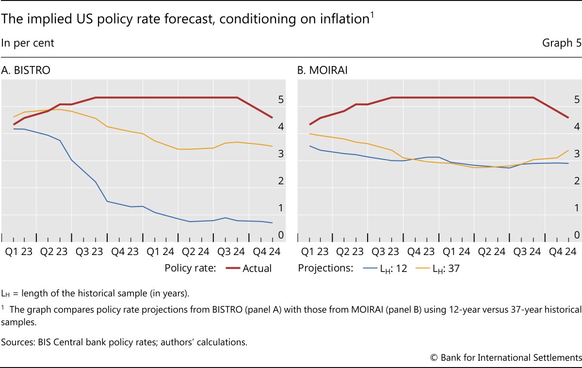
Results crucially depend on the amount of historical information we condition on (Graph 5). When conditioning only on the last 12 years of data in our sample (eg 2011–22), the model uses information based on a low-inflation regime in which monetary policy was mostly conducted through unconventional tools, due to the effective lower bound. Hence, the link between policy rates and inflation appears quite weak. As a result, the model fails to recognise that a policy tightening is necessary to tame inflation and instead hints at near-zero policy rates, implicitly assuming that inflation would self-correct without the need for policy intervention.

If one instead extends the context window to cover the entire training sample (1986–2022), the model gains exposure to different inflationary regimes and to a phase in which conventional policy played a key role keeping inflation in check. In this richer context, the model correctly infers that high inflation typically calls for a tightening of policy rates, leading to a somewhat sharper rise in the implied interest rate path that slightly exceeds the realised pace of tightening in the very beginning. By contrast, the projections generated by MOIRAI are largely insensitive to the length of the conditioning history, yielding similar policy rate paths across the two settings. This contrast suggests that BISTRO makes more effective use of historical information when capturing the correlations between inflation and monetary policy.

Opening the black box: the role of the attention weights

The different performances of BISTRO and MOIRAI in dealing with covariates and conditional scenarios underscore the key role played by the attention weights. While BISTRO's attention weights effectively integrate covariate data to generate meaningful scenarios, MOIRAI fails to assimilate this information, resulting in less informative projections.

To explain why this is so, let us first focus on MOIRAI. As illustrated in Graph 4.B, MOIRAI's predictions remain unchanged across the four distinct oil price scenarios. This suggests that the attention weights assigned to the oil price time series are effectively zero, therefore the model ends up relying entirely on historical inflation data. Consequently, MOIRAI is unable to infer the relationship between inflation and oil prices from past observations. Furthermore, Graph 5.B demonstrates that the predicted policy rate differs only marginally when contrasting short and long historical contexts. This implies that MOIRAI predominantly relies on the most recent readings, largely disregarding earlier values of both the policy rate and inflation.

In contrast, BISTRO, having been specifically trained on macroeconomic time series data, demonstrates an ability to assign attention weights that capture relevant historical information. In Graph 4.A, the model's non-linear attention weights successfully reflect the complex, non-linear impact of oil prices on inflation. Additionally, as shown in Graph 5.A, BISTRO leverages longer time horizons by assigning greater attention to observations from the more distant past, thereby enhancing its policy rate projections. This adaptability of the transformer model, whereby it can refine its estimates by adjusting attention weights, rather than requiring retraining, underscores its strength as a general purpose forecasting tool. Nevertheless, this also highlights the necessity for the model to be exposed to time series pertinent to the specific forecasting task.

Concluding remarks

The key advantage of BISTRO compared with alternatives lies in its flexibility. It can accommodate prediction of a multitude of time series in unconditional as well as conditional terms. Importantly, it is also able to unveil and deal with non-linearities. While we provided a few examples, BISTRO lends itself to plenty of different empirical exercises, ranging from pure forecasting to scenario analysis.

References

Alammar, J (2018): "The illustrated transformer", June, https://jalammar.github.io/illustrated-transformer/.

Aldasoro, I, P Hoerdahl, A Schrimpf and S Zhu (2025): "Predicting financial market stress with machine learning", BIS Working Papers, no 1250, March.

Ansari, A F, O Shchur, J Küken, A Auer, B Han, P Mercado, S S Rangapuram, H Shen, L Stella, X Zhang, M Goswami, S Kapoor, D Maddix, P Guerron, T Hu, J Yin, N Erickson, P M Desai, H Wang, H Rangwala, G Karypis, Y Wang and M Bohlke-Schneider (2025): "Chronos-2: from univariate to universal forecasting", arXiv:2510.15821, October.

Aquilina, M, D Araujo, G Gelos, T Park and F Perez-Cruz (2025): "Harnessing artificial intelligence for monitoring financial markets", BIS Working Papers, no 1291, September.

Bank for International Settlements (BIS) (2024): "Artificial intelligence and the economy: implications for central banks", Annual Economic Report, Chapter III, June.

Brown, T, B Mann, N Ryder, M Subbiah, J Kaplan, P Dhariwal, A Neelakantan, P Shyam, G Sastry, A Askell, S Agarwal, A Herbert-Voss, G Krueger, T Henighan, R Child, A Ramesh, A Ziegler, J Wu, C Winter, C Hesse, M Chen, E Sigler, M Litwin, B Gray, B Chess, J Clark, C Berner, S McCandlish, A Radford, I Sutskever and D Amodei (2020): "Language models are few-shot learners", Advances in Neural Information Processing Systems, vol 33.

Cao, S, W Jiang, J L Wang and B Yang (2024): "From man vs. machine to man + machine: the art and AI of stock analyses", Journal of Financial Economics, vol 160, no 103910.

Carriero, A, D Pettenuzzo and S Shekhar (2024): "Macroeconomic forecasting with large language models", arxiv.org 2407.00890, July.

Faria-e-Castro, M and F Leibovici (2024): "Artificial intelligence and inflation forecasts", Federal Reserve Bank of St. Louis Review, vol 106, no 12.

Faust, J and J H Wright (2013): "Forecasting inflation", Handbook of Economic Forecasting, vol 2, part A, chapter 1.

Gambacorta, L, B Kwon, T Park, P Patelli and S Zhu (2024): "CB-LMs: language models for central banking", BIS Working Papers, no 1215, October.

Gorodnichenko, Y, T Pham and O Talavera (2023): "The voice of monetary policy", American Economic Review, vol 113, no 2.

Hall, S, G Tavlas and Y Wang (2023): "Forecasting inflation: the use of dynamic factor analysis and nonlinear combinations", Journal of Forecasting, vol 42, no 3.

Hendry, D and H-M Krolzig (2001): Automatic econometric model selection using PcGets 1.0, Timberlake Consultants Press.

Horton, J (2023): "Large language models as simulated economic agents: what can we learn from Homo Silicus?", NBER Working Papers, no 31122, April.

Korinek, A (2023): "Generative AI for economic research: use cases and implications for economists", Journal of Economic Literature, vol 61, no 4.

----- (2025): "AI agents for economic research", NBER Working Papers, no 34202, September.

Koyuncu, B, B Kwon, M Lombardi, F Perez-Cruz and H S Shin (2026): "Introducing BISTRO: a foundational model for unconditional and conditional forecasting of macroeconomic time series", BIS Working Papers, forthcoming.

Kwon, B, T Park, F Perez-Cruz and P Rungcharoenkitkul (2024): "Large language models: a primer for economists", BIS Quarterly Review, December.

Kwon, B, T Park, P Rungcharoenkitkul and F Smets (2025): "Parsing the pulse: decomposing macroeconomic sentiment with LLMs", BIS Working Papers, no 1294, October.

Ludwig, J and S Mullainathan (2024): "Machine learning as a tool for hypothesis generation", Quarterly Journal of Economics, vol 139, no 2.

Radford, A and K Narasimhan (2018): "Improving language understanding by generative pre-training", OpenAI, mimeo.

Radford, A, J Wu, R Child, D Luan, D Amodei and I Sutskever (2019): "Language models are unsupervised multitask learners", OpenAI, technical report.

Siano, F (2025): "The news in earnings announcement disclosures: capturing word context using LLM methods", Management Science, vol 71, no 11.

Vaswani, A, N Shazeer, N Parmar, J Uszkoreit, L Jones, A N Gomez, Ł Kaiser and I Polosukhin (2017): "Attention is all you need", Advances in Neural Information Processing Systems, vol 30.

Woo, G, C Liu, A Kumar, C Xiong, S Savarese and D Sahoo (2024): "Unified training of universal time series forecasting transformers", ICML'24: proceedings from the 41st International Conference on Machine Learning, article no 2178.

Zarifhonarvar, A (2026): "Generating inflation expectations with large language models", Journal of Monetary Economics, vol 157(C).

Footnotes

¹   The views expressed in this publication are those of the authors and not necessarily those of the BIS or its member central banks. We also thank Jon Frost, Gaston Gelos, Denis Gorea, Benoit Mojon, Matthias Rottner, Phurichai Rungcharoenkitkul, Dan Rees, Andreas Schrimpf, Frank Smets and Sonya Zhu for helpful comments and suggestions.

²   Early proposals of automatic and flexible modelling for time series (Hendry and Krolzig (2001)) hinged on a necessarily task-specific model selection step.

³   Korinek (2023) surveys how generative AI can support economic research, while Korinek (2025) explores specific applications, including the replication of existing results.

⁴   See for example Aldasoro et al (2025), Aquilina et al (2025); Cao et al (2024); Gambacorta et al (2024); Gorodnichenko et al (2023); Horton (2023); Kwon, Park, Perez-Cruz and Rungcharoenkitkul (2024); Kwon, Park, Rungcharoenkitkul and Smets (2025); Ludwig and Mullainathan (2024); Siano (2025); and Zarifhonarvar (2026).

⁵   The transformer architecture is a deep neural network originally developed for language translation. For further details, see Vaswani et al (2017). GPT was introduced by Radford and Narasimhan (2018) and further evaluated in Radford et al (2019) and Brown et al (2020).

⁶   Vaswani et al (2017) introduced the attention mechanism for transformers, and Alammar (2018) subsequently elucidated its inner workings; see the Annex for further details.

⁷   Chronos 2.0 (Ansari et al 2025) is another foundational model comparable to MOIRAI. Carriero at al (2024) compare the performance of several univariate off-the-shelf foundational models for macroeconomic forecasting.

⁸   Fine-tuning a foundational time series model is analogous to the process that turns a general purpose language model into a practical assistant, such as ChatGPT, Claude or Gemini. In that context, fine-tuning adjusts the model's parameters so that it responds conversationally, filters out unreliable information prevalent in its original training data and adopts a style suited to its users.

⁹   For simplicity, we abstract from data revisions. While revisions are an important issue for GDP, most other macroeconomic time series are revised only sporadically and by small amounts.

¹⁰ Despite their simplicity, autoregressive models are a tough benchmark to beat when forecasting macroeconomic aggregates. See for example Faust and Wright (2013) and Hall et al (2023).

¹¹ Admittedly, this period was also included in the training sample. Yet note that in the training of the model, the inflation time series was never presented in isolation or explicitly labelled as "inflation", and it was expressed in month-on-month rather than year-on-year terms. Furthermore, the only information available to the model consisted of the numerical values within the time series. Had the model memorised the time series exactly, it would have perfectly replicated the forthcoming surge in inflation. That said, later in the article we also run a full-fledged forecasting comparison using forecasting windows that were deliberately excluded from the training sample.

¹² Faria-e-Castro and Leibovici (2024) employ a text-based LLM to predict the 2021 US inflation surge, achieving results comparable to AR(1) predictions.

¹³ To ensure comparability across models, we apply the same principle to the AR(1) benchmark, whose coefficients are not iteratively re-estimated throughout the test period.

¹⁴ For a detailed breakdown of the results, see Koyuncu et al (2026).

¹⁵ This is partly because BISTRO makes quite large errors compared with the AR(1) benchmark for the United Kingdom and New Zealand in the 2023–24 test window.