Large language models: a primer for economists

Large language models (LLMs) are powerful tools for analysing textual data, with substantial untapped potential in economic and central banking applications. Vast archives of text, including policy statements, financial reports and news, offer rich opportunities for analysis. This special feature provides an accessible introduction to LLMs aimed at economists and offers applied researchers a practical walkthrough of their use. We provide a step-by-step guide on the use of LLMs covering data organisation, signal extraction, quantitative analysis and output evaluation. As an illustration, we apply the framework to analyse perceived drivers of stock market dynamics based on over 60,000 news articles between 2021 and 2023. While macroeconomic and monetary policy news are important, market sentiment also exerts substantial influence.¹

JEL classification: C55, C63, G10

Large language models (LLMs) represent a breakthrough application of machine learning techniques to natural language processing (NLP). Machine learning algorithms excel at imposing mathematical structure on unstructured data. They do so by converting text, speech or images into arrays of numbers, ie vectors. This "embedding" process has a wide variety of applications, as it transforms complex unstructured data into structured data suitable for mathematical operations and statistical analysis. LLM techniques can support many use cases, such as forecasting, nowcasting and surveillance, as well as sentiment analysis of news, social media and policy reports. For economists and central bankers accustomed to working with structured numerical data, LLMs are powerful additions to their toolkit.

This primer offers accessible guidance on LLM technologies and highlights key considerations for economists.² We cover topics such as model selection, pre-processing techniques, topic modelling, quantitative analysis and the involvement of human judgment. The guide is tailored to use cases commonly encountered by central bankers but with a wide applicability in any social science field that works with text data. To showcase the practical usage, we apply our guidelines to analyse perceived drivers of US equity prices, with accompanying sample code available in a GitHub repository. An online glossary provides definitions of key technical terms.

We first introduce key technologies that underpin LLMs. We then present a stylised workflow for their application, highlighting best practices and common pitfalls. Next, we show how to implement this workflow in a concrete exercise by isolating perceived drivers of US stock market movements. And finally we conclude.

Introduction to large language models

The central idea

Machine learning techniques excel at imposing mathematical structure on unstructured data. In the NLP context, this entails projecting words into a vector space – a process called embedding. Relationships between words are then represented by their Euclidean distance in the vector space, with a smaller distance indicating a closer semantic relationship. The word embedding for "football" is closer to "basketball" and further from "monsoon", which is closer to "cloud". These embeddings allow the use of algebraic techniques to convey relationships between words (see BIS (2024)). For example, the embeddings for countries and capitals would obey: = - + , consistent with the notion that Seoul is related to Korea in the same way that Madrid is related to Spain. Similarly, simple linear algebra applies, eg - = - Furthermore, embeddings for sentences, paragraphs or any group of words can be computed as a weighted sum of the word embeddings to represent their collective meaning (Arora et al (2017)). Embeddings pave the way for applying mathematical tools to languages, enhancing tasks such as sentiment analysis, translation, sentence completion and named-entity recognition (eg recognising the Bank for International Settlements as a single unit rather than four separate words). This mapping of textual data into numerical form using embeddings is essential for any subsequent analysis.

Early neural networks³ for NLP (eg Word2vec (Mikolov et al (2013)) assigned a single unique vector to each word. These methods, which were significant advancements at the time, have been extensively utilised by economists since their inception.⁴ However, this one-to-one mapping suffers from an important drawback – it cannot recognise the meanings of words that vary with context. It might struggle with a sentence such as "The bank raises rates to lower inflation." Inferring correctly that "bank" refers to the "central bank" rather than a riverbank or a commercial bank requires taking into account the words that give context in this sentence, namely "raises" and "rates".

What gives LLMs an edge over earlier NLP methods is a neural network known as the transformer architecture (Box A). This breakthrough creates a word embedding based on its context, allowing the embedding to capture the word's meaning within the overall context of the surrounding text rather than just its dictionary form.⁵ For example, the transformer architecture would place embeddings for "bank" (financial) and "money" closer together because they frequently appear in similar contexts, while "bank" (river) would be positioned further away from "money" and closer to "meadow". Additionally, LLMs account for word sequences in sentences, enabling them to clearly distinguish between "The bank raises rates to lower inflation" and "The bank lowers rates to raise inflation."

The techniques

The original transformer for translation included two components: an encoder, which transforms input language into an embedding vector, and a decoder, which converts the embedding into output language. Current LLMs draw on one of the two – the encoder as in bidirectional encoder representations from transformer (BERT) or the decoder as in generative pretrained transformer (GPT). Each has its own strengths. GPT sequentially uses each word's preceding text to create its contextualised embedding and can be used to generate text. This self-generating process is similar to how an autoregressive model is capable of making recursive forecasts. In contrast, BERT uses both preceding and subsequent words taken together to create the embedding for each word. It is akin to using the full sample to draw econometric inferences. GPT is more widely recognised but is not necessarily superior for all tasks. In many economic applications, BERT may be more suitable for quantitative analysis because it uses subsequent text to infer context (eg Gambacorta et al (2024)).

Economists can deploy LLMs to analyse vast amounts of text data more accurately and efficiently. LLMs are not a blank slate, as their parameters have been previously estimated with massive data sets downloaded from the internet - a process commonly known as pretraining. Economists can directly use these pretrained models to embed text for analysis. Alternatively, they can re-estimate or modify the LLM parameters using their economic text data, much like with any econometric model. This process, known as fine-tuning, adjusts the LLM to the specific economic data and research questions, yielding more accurate and relevant predictions.

Instead of fine-tuning, economists can also use the chatbot version of an LLM (eg ChatGPT, Claude, Gemini, etc) and ask the question directly through the chat interface or via an application programming interface (API). This approach does not modify model parameters but allows users to obtain improved responses by providing more context and guidance through prompting, known as in-context learning (Box B). Although this approach allows the convenient use of plain English or any other natural language, managing the consistency and quality of responses for robust research output can be challenging.

Putting LLMs to work

To show how to put LLMs to work, we lay out a step-by-step workflow analogous to that of an econometrician and discuss how LLM tools can enhance capabilities in analysing unstructured text data at scale.⁶ The workflow includes the following steps:

1. Data organisation: Just as an economist begins an empirical project by collecting and cleaning data, an analysis of text starts with text retrieval, pre-processing and, additionally, vector embedding.

2. Signal extraction: The next step is to extract key informational content from the data, similar to principal component analysis (PCA) or trend filtering in econometrics. This is important because the embedding vectors from the previous step have many dimensions (eg 4,096 for Llama 3.1 8B) and are too complex to analyse. Hence, some dimensionality and complexity reduction are necessary. Topic modelling is a powerful tool to do this, by organising text into common themes while respecting the context.

3. Quantitative analysis: In this step, the researcher engages in quantitative modelling and analysis. Sentiment analysis is one common tool for measuring intent, tone and opinions from text and can be assisted by LLMs to identify meaningful labels or scores. Standard statistical methods such as regression may also be applied directly to embeddings or sentiment scores produced by LLMs.

4. Outcome evaluation: The last step is to evaluate the model's output, eg based on the out-of-sample prediction as in standard econometrics. Here, text data raise unique challenges.

We consider each of the above steps in more detail.

Data organisation

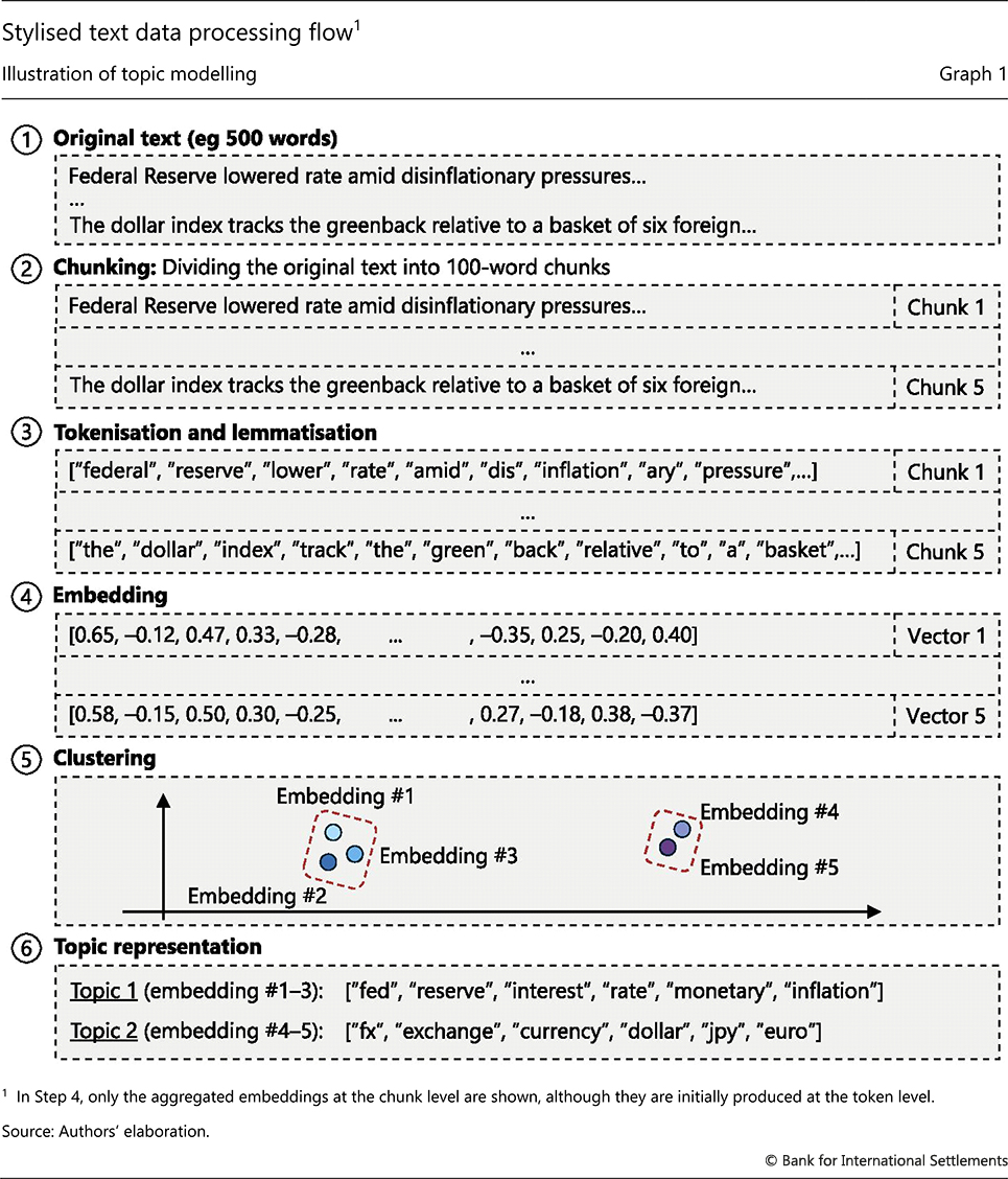
The objective of this step is to gather relevant text data and prepare them for contextualised embedding through text cleaning. The pertinent sources may be central bank statements, governors' speeches, policy papers, news articles or any other text sources. The next step is to divide the documents into so-called "chunks" of words, ie text segments of words, to prepare for embeddings (step 2 of Graph 1).⁷ Each chunk serves as a unit of text analysis. The chunk size strikes a balance between breadth and granularity. It should be long enough to capture the relevant information and context, but not so long as to collapse a large block of text into a single vector and lose the nuances of different messages.

The next step involves breaking words down to their root forms to simplify the task of LLM embeddings. Tokenisation is a process of breaking words down into smaller units called tokens; lemmatisation in turn simplifies words to their base forms to focus on their core meanings (step 3 of Graph 1). For example, tokenisation breaks the word "disinflationary" down into three tokens: "dis-" (prefix), "inflation" (base word) and "-ary" (suffix). Lemmatisation assigns "lowered" to "lower", "pressures" to "pressure" and "tracks" to "track". Each LLM has its own set of rules for tokenising and lemmatising words.⁸ Researchers need to apply appropriate tokenisation rules that are compatible with their selected LLM.

Once all text chunks have been tokenised and lemmatised, one can proceed to generating the embeddings (step 4 of Graph 1). If using a BERT-like (encoder) model, one will generate a global embedding for the entire chunk, called the classification (CLS) embedding. If using a GPT-based (decoder) model, the embedding for the text chunk can be obtained as a weighted sum of each word's embedding (Arora et al (2017)). In either case, one can rely on embedding models that have been trained by tech companies such as Anthropic, Google, Meta, Mistral AI or OpenAI. Alternatively, one could modify these models using own data⁹ to tailor the embeddings to research objectives. This domain-adaptation option is naturally more costly and is only advisable if sufficient data and computational resources are available. Additionally, the recent state-of-the-art LLMs are often sufficiently trained with economic terms, lessening the need for additional training.

Signal extraction

The second step aims to extract signals and distil key information from the retrieved text data through dimensionality reduction. It simplifies high-dimensional embedding vectors by extracting only the most relevant information needed for meaningful interpretation, thus improving computational efficiency. In LLM analysis, potential tools include topic modelling, clustering techniques or embedding-based dimensionality reduction, such as Uniform Manifold Approximation and Projection (UMAP) (McInnes et al (2018)). These methods facilitate the formation of clusters of embeddings obtained from the previous step (step 5 of Graph 1).

We focus on topic modelling due to its broad applicability, where the objective is typically to extract the main messages from text data. Traditional topic modelling tools, such as latent Dirichlet allocation (LDA) (Blei et al (2003)), do this by grouping keywords under common themes but cannot differentiate between nuanced subtopics or contextual shifts within the same overarching theme. With LLMs, topic modelling leverages the transformer architecture and embeddings to provide a context-sensitive representation of text in identifying the dominant themes.

Topic modelling can be unsupervised, allowing the data to reveal patterns autonomously, or supervised, where prior knowledge or guidance shapes the output.

Unsupervised topic modelling summarises the dominant themes in text through keyword lists, offering a high-level overview of key topics without relying on pre-defined classification schemes. A common procedure, such as BERTopic (Grootendorst (2022)), starts by generating embeddings for each text chunk. The algorithm then groups contextually similar embeddings into clusters, typically after applying dimensionality reduction to enhance efficiency and performance (see step 5 of Graph 1). After completing this step, a researcher may assign a topic label – a few keywords – that best represents the cluster. These labels are often selected manually from the original list of keywords associated with the cluster, both reflecting the researcher's focus and interests and ensuring clear differentiation between clusters. For example, in step 6 of Graph 1, one might label Topic 1 as "monetary policy" and Topic 2 as "FX markets".

A potential drawback of unsupervised topic modelling is that it may generate topics irrelevant to the researcher's focus. For example, when analysing stock markets, names of major stocks or asset management firms might dominate because they are frequent within a specific cluster and distinct from those in other clusters. This may not be of interest to a macro-finance researcher who wants to study monetary policy and market valuations. As a result, unsupervised methods often require post-processing to align the topics with specific research goals – a practice we follow in the application below.

Resorting to supervised topic modelling avoids generating irrelevant topics, as it allows researchers to define topics of interest from the outset. One common option is seeding, where a set of relevant terms is introduced to guide the topic modelling process. For example, providing keywords related to monetary policy (eg "Federal Reserve", "policy rates", "FOMC Chair") directs the model to focus on text segments that are semantically closest to the concept of monetary policy.

Quantitative analysis

Once the text data have been converted into vectors and organised by topics, they are ready for use in quantitative analysis. As the embeddings are in vector format, researchers can employ standard econometric tools such as panel regressions for classification data or autoregressions for time-stamped text. In the illustration that follows, we focus on sentiment analysis. This is one of the most relevant problems in economics and social science when the data are only in text form.

Sentiment analysis assigns predefined labels to each text chunk. Classification could be binary (positive or negative), tertiary (positive, neutral or negative) or more multidimensional.¹⁰ Without an LLM, this transformation may need to rely on a dictionary of terms compiled by the researcher to map a chosen list of words reflecting tones to sentiments. This approach is laborious and prone to errors and risks false assignments when context is important.

Depending on the application, one can analyse sentiment either at the small chunk level (local analysis) or globally across the entire document. The chunk size sets the level of granularity: smaller chunks allow for different passages in an article to convey different sentiments. In some cases, capturing local sentiment may be more advisable, as the goal may be to uncover different aspects of the unfolding of a story. For instance, both positive and negative forces weighing on the stock market could be described in the same document. In other cases, the document's overall message may be where the researcher's interest lies. For instance, in monetary policy statements, the overall assessment and final decision may matter the most, justifying document-level sentiment analysis.

The choice of language models for sentiment analysis depends on many factors. These include task complexity, text volume, the availability of labelled training data, computing capacity, expertise and the time required for manual labelling. Among sentiment analysis tools, pretrained encoder-based models such as BERT (Devlin et al (2018)) and RoBERTa (Liu et al (2019)) offer a suitable architecture for most applications. These models are specifically designed to encode contextual information, excel at capturing the sentiments of input text and are fast to run. For highly specialised applications, specifically trained LLMs can be more effective. For instance, the "CB-LMs" of Gambacorta et al (2024) are trained on central banking documents and may be better at capturing central banking nuances than general models. As for decoder-based GPT models, their extremely large sizes are key advantages, though their architecture may not be ideal for sentiment classification and they tend to have a longer runtime.

If the researcher opts for BERT-based LLMs, they will need to conduct fine-tuning to help the model learn how to classify embeddings. This requires a labelled data set (eg assigning positive, neutral and negative to a portion of the data as training examples). During fine-tuning, the model is further trained on this labelled data set in a supervised learning process to classify sentiments in the embedding space (Devlin et al (2018)). The process updates both the embeddings themselves and the boundaries separating different sentiments, making it easier for the model to correctly classify sentiments of new text inputs.

If the researcher adopts GPT-based models which have been trained with a large amount of data, such as state-of-the-art chatbots, fine-tuning is often unnecessary and not worthwhile.¹¹ In many cases, low-effort in-context learning can be sufficient (see Box B and Gambacorta et al (2024)). These models typically require minimal or no data preprocessing, such as tokenisation or embedding. Researchers can directly input text for topic modelling and sentiment analysis using common language instructions.

Outcome evaluation

LLMs, as a machine learning tool, are best evaluated by their predictive performance. For example, in classification problems, the objective could be to minimise the misclassification error. Note that usual statistical principles such as parsimony or statistical significance of coefficients do not apply in a machine learning context. Modern LLMs do in fact have hundreds of billions of parameters and embedding vectors with a few thousand elements. The main focus is on making accurate predictions in the test set, with overfitting concerns addressed by various techniques (eg regularisation, initialisation and stochastic gradient descent).

In evaluating performance, researchers should choose error measures that align with their applications and desired outcomes. For example, in regression with outlier problems, absolute errors might be preferable to squared errors. Or when the outcome spans several orders of magnitude, measuring errors in the logarithm of the output may help reduce the relative error. For problems with imbalanced classes and uneven costs for false positives and false negatives, the F1 score¹² is often an appropriate metric, as it trades off "precision" and "recall" in classification. Precision measures how many predicted positive examples are positive, while recall captures how many positive examples are correctly identified by the model. Combining the two helps control both false positives and false negatives.

Illustration in a study of equity market drivers

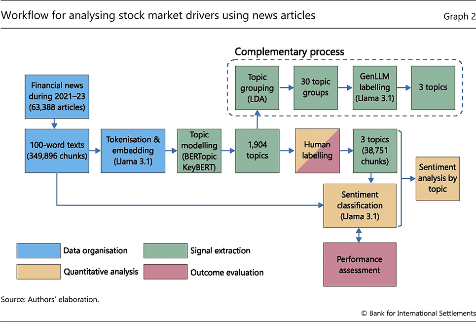
We now illustrate how to operate the workflow in a concrete project. The objective is to identify perceived drivers of stock market prices using news reports. The sample includes 63,388 daily news articles published over 2021–23, from sources such as the Wall Street Journal, Reuters, Forbes and MarketWatch. The sample period covers a sharp monetary policy tightening and a surge in inflation. Graph 2 summarises the overall workflow.

Data organisation

We start by retrieving news articles from Factiva and use its topic tagging to select articles potentially relevant to the US stock markets, as measured by their performance in the S&P 500. We split each of the 63,388 articles into chunks of 100 words to capture localised context, producing 349,896 text chunks.¹³ We transform each chunk using the Llama 3.1 8B, which embeds each word in the chunk into a 4,096-dimensional vector. To summarise the key messages of each chunk, we then average over the 100-word embeddings, to obtain a 4,096-dimensional vector embedding representing the whole chunk.¹⁴

Signal extraction

We next employ BERTopic to assign text chunk embeddings to initial topics. As the initial output contains several irrelevant topics, some filtering is necessary. A significant portion of the chunks (190,477) are dropped, as they do not relate to any specific topic clusters¹⁵ and instead cover general topics (eg economy, policy, market, etc). Additionally, we filter out chunks that belong to a cluster but are only loosely associated. We also exclude clusters with too few articles.

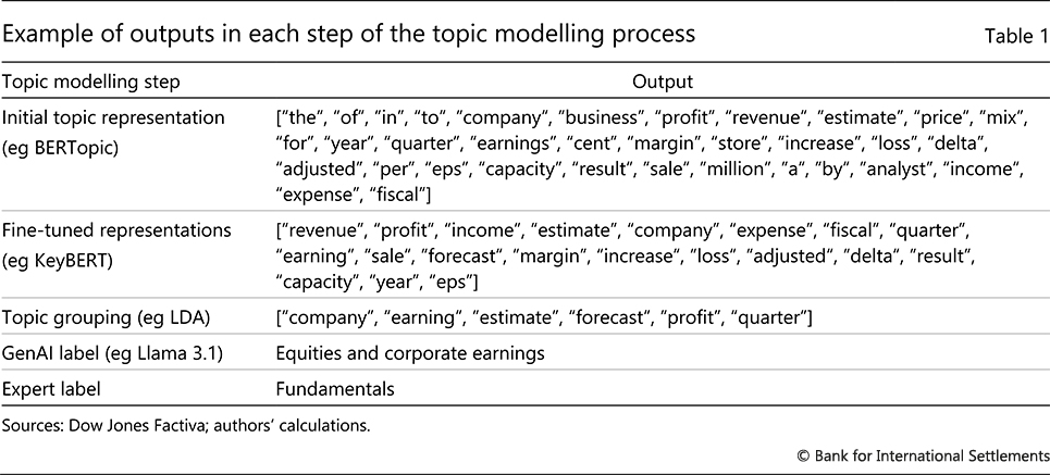
To further refine the topic sets, as illustrated in Table 1, we apply KeyBERT (Grootendorst (2020)) to extract meaningful keyword sets from the BERTopic results and filter out less relevant terms. We then merge the refined keyword sets using LDA,¹⁶ reducing the nearly 2,000 topics into a smaller, more manageable set of keyword clusters. LDA allows us to analyse the topics within broader themes.¹⁷

To assign intuitive and descriptive labels to the topics, we use Llama 3.1 to generate initial labels based on the grouped keyword sets. One could also apply Llama 3.1 from the initial step of topic modelling. That said, as discussed, the large input size and computational overhead pose a constraint. Additionally, maintaining control over the process ensures more effective and transparent topic labelling.

Finally, we review the topics and make final manual adjustments to ensure the labels and groupings are contextually meaningful and aligned with research objectives. The initial topic grouping performed by LDA, along with the labelling provided by Llama 3.1, facilitates this process. After reviewing, we categorise the news articles into three broad topics: fundamentals (with KeyBERT keywords such as "profit", "economy" and "employment"), monetary policy ("fed" and "interest rate"), and market sentiment ("overbought", "buzz", "volatility" and "ipos").

This classification into three topics mirrors common analytical approaches to stock price analysis. First, stock prices are determined by current and expected future dividends (fundamentals). These are adjusted by the discount rate, which depends on the risk-free interest rate (monetary policy) as well as a compensation for risk that reflects investor risk appetite and sentiment (market sentiment).

Topic modelling reduces the data set to just 10% of its original size, resulting in a final output of 38,751 targeted text chunks, assigned to the three categories: fundamentals (16,879), market sentiment (14,468) and monetary policy (7,404).

Quantitative analysis and outcome evaluation

After classifying news article texts into the three topics, we conduct sentiment analysis within each topic. We use the Llama 3.1 70B model¹⁸ to classify each topic in each news chunk as either negative, neutral or positive (with scores –1, 0 and 1), with positive indicating an association with stock price increases. In doing so, we employ few-shot learning and provide task-specific instructions and examples for each topic.¹⁹ We then sum the scores across all article chunks to derive the aggregate sentiment score corresponding to each topic.

Results

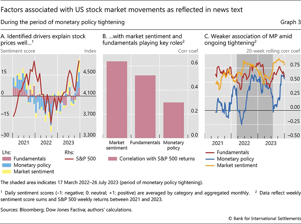
The aggregate sentiment score aligns well with stock market movements (Graph 3.A). This suggests that the procedure is extracting the appropriate signals from text data. Examining the relative importance of sentiment scores across the three categories, "market sentiment" and "fundamentals" co-move the most with the stock returns, showing correlation coefficients of 0.64 and 0.52, respectively (Graph 3.B).

The association between monetary policy sentiment and stock market performance is more tenuous, with a correlation of 0.30. Despite this period being one of the most aggressive monetary tightening episodes in recent history, the stock market – aside from the large drawdown in 2022 – held up well. One possible interpretation is that strong "fundamentals", and hence associated positive "market sentiment", may have offset the dampening effect of "monetary policy" tightening on stock returns.

Over the sample, the relationship between monetary policy sentiment and stock market performance has seen notable fluctuations, unlike market sentiment and fundamental factors. The correlation between monetary policy sentiment and stock returns rose to its highest point of over 0.6 in 2022, coinciding with the most active monetary policy tightening. But once the tightening stopped, the correlation between monetary policy sentiment and stock returns declined (Graph 3.C). The result is consistent with the broader disconnect between financial conditions and the monetary policy stance in recent years, as documented elsewhere. ²⁰

Final considerations

Our stylised workflow offers broad lessons on general principles and best practices in making the most of LLMs. One is careful resource planning. While extremely powerful, the use of LLMs can be computationally expensive. Some of the computational steps, such as working with high-dimensional embeddings or the largest LLMs, may be run at most a few times in practice. This also means good research design is critical. For example, condensing input text data, as we do using topic modelling, helps reduce unnecessary computational load and improve model performance by focusing resources on the most relevant tasks. More generally, adopting a modular step-by-step process would enable researchers to check and analyse intermediate outputs, ensuring that the LLM procedure produces sensible outcomes as intended. Finally, given the probabilistic nature of LLM algorithms, some repetition of the procedures would help ensure robustness, if at additional computational costs.

Another important consideration pertains to data privacy and confidentiality. Researchers must ensure compliance with relevant regulations, such as corporate policies, data licences or other data protection laws. Using locally hosted LLMs, instead of cloud-based ones, may mitigate risks to some extent but not entirely, as some regulations apply regardless of the hosting environment.

The vast power of LLMs is best harnessed when researchers both understand and manage the models' limitations effectively. Recognising and addressing potential biases is essential at each stage of the analysis to ensure a successful application. As LLMs are in essence statistical models, it is up to users to apply informed judgment in evaluating outputs. The synergy between human oversight and LLM capabilities can help enhance quality control while mitigating potential risks, leading to more robust outcomes.

References

Alammar, J (2018): "The illustrated transformer", blog post, available at jalammar.github.io/illustrated-transformer/.

Araujo, D, S Doerr, L Gambacorta and B Tissot (2024): "Artificial intelligence in central banking", BIS Bulletin, no 84, January.

Arora, S, Y Liang and T Ma (2017): "A simple but tough-to-beat baseline for sentence embeddings", in Proceedings of the 5th International Conference on Learning Representations, Toulon, France, 24–26 April.

Athey, S and G W Imbens (2019): "Machine learning methods that economists should know about", Annual Review of Economics, vol 11, pp 685–725, August.

Bank for International Settlements (2024): Annual Economic Report, June.

Blei, D, A Ng and M Jordan (2003): "Latent Dirichlet allocation", Journal of Machine Learning Research, vol 3, pp 993–1022.

Brown, T, B Mann, N Ryder, M Subbiah, J Kaplan, P Dhariwal, A Neelakantan, P Shyam, G Sastry, A Askell, S Agarwal, A Herbert-Voss, G Krueger, T Henighan, R Child, A Ramesh, D Ziegler, J Wu, C Winter, C Hesse, M Chen, E Sigler, M Litwin, S Gray, B Chess, J Clark, C Berner, S McCandlish, A Radford, I Sutskever and D Amodei (2020): "Language models are few-shot learners", arXiv, no 2005.14165 [cs.CL].

Cho, A, G Kim, A Karpekov, A Helbling, J Wang, S Lee, B Hoover and P Chau (2024): "Transformer explainer", arXiv, no 2408.04619, available at poloclub.github.io/transformer-explainer/.

Dell, M (2024): "Deep learning for economists", arXiv, no 2407.15339v1 [econ.GN], July.

Devlin, J, M-W Chang, K Lee and K Toutanova (2018): "BERT: pre-training of deep bidirectional transformers for language understanding", arXiv, no 1810.04805 [cs.CL].

Gambacorta, L, B Kwon, T Park, P Patelli and S Zhu (2024): "CB-LMs: language models for central banking", BIS Working Papers, no 1215, October.

Grootendorst, M (2020): "KeyBERT: minimal keyword extraction with BERT", Zenodo, version v0.3.0, doi.org/10.5281/zenodo.4461265.

Grootendorst, M (2022): "BERTopic: neural topic modeling with a class-based TF-IDF procedure", arXiv, no 2203.05794 [cs.CL].

Korinek, A (2023): "Generative AI for economic research: use cases and implications for economists", Journal of Economic Literature, vol 61, no 4, pp 1281–1317, December.

Korinek, A (2024): "LLMs level up-better, faster, cheaper: June 2024 update to Section 3 of 'Generative AI for Economic Research: Use Cases and Implications for Economists'", published in the Journal of Economic Literature, vol 61, no 4.

Liu, Y, M Ott, N Goyal, J Du, M Joshi, D Chen, O Levy, M Lewis, L Zettlemoyer and V Stoyanov (2019): "RoBERTa: a robustly optimized BERT pretraining approach", arXiv, no 1907.11692 [cs.CL].

Matsui, A and E Ferrara (2022): "Word embedding for social sciences: an interdisciplinary survey", arXiv, no 2207.03086 [cs.AI].

McInnes, L, J Healy and J Melville (2018): "UMAP: uniform manifold approximation and projection for dimension reduction", arXiv, no 1802.03426 [stat.ML].

Mikolov, T, K Chen, G Corrado and J Dean (2013): "Efficient Estimation of Word Representations in Vector Space", arXiv, no 1301.3781 [cs.CL].

Vaswani, A, N Shazeer, N Parmar, J Uszkoreit, L Jones, A Gomez, L Kaiser and I Polosukhin (2017): "Attention is all you need", arXiv, no 1706.03762 [cs.CL].

Wei, J, X Wang, D Schuurmans, M Bosma, V Chi, Q Le, E Chi and D Zhou (2022): "Chain-of-thought prompting elicits reasoning in large language models", arXiv, no 2201.11903 [cs.CL].

¹   The views expressed are not necessarily those of the Bank for International Settlements. For helpful comments, we are grateful to Douglas Araujo, Claudio Borio, Leonardo Gambacorta, Gaston Gelos, Benoît Mojon, Andreas Schrimpf, Hyun Song Shin and Kevin Tracol. All remaining errors are ours.

²   Our focus on practical implementation complements recent reviews such as Araujo et al (2024), Athey and Imbens (2019), Dell (2024) and Korinek (2023, 2024).

³   A neural network is a function that maps inputs to outputs through layers of matrix multiplications and a component-wise non-linear function that can provide a tight fit across a variety of tasks.

⁴   See Matsui and Ferrara (2022) and the references therein.

⁵  Originally proposed for translation (Vaswani et al (2017)), the transformer removes bottlenecks in previous architectures by processing data in parallel, increasing speed by several orders of magnitude.

⁶   Researchers could readily extend this analysis to images and audio too.

⁷   Dividing text data into blocks of words – eg several hundred words as a proxy for a paragraph – is often easier to program and hence more practical than differentiating sentences or paragraphs.

⁸  For examples, see the OpenAI Platform Tokenizer at platform.openai.com/tokenizer or the Lunary Llama 3 Tokenizer at lunary.ai/llama3-tokenizer.

⁹   Training these models with private data is not advisable if the models are available for widespread use, as they may memorise the training data.

¹⁰  One example is to capture the intensity and nuances of opinions expressed in economic or financial discourse. For instance, in analysing central bank communication, one can detect degrees of confidence and uncertainty about the economic outlook beyond binary classification.

¹¹  Fine-tuning GPT-based models is computationally demanding and generally does not improve performance over fine-tuning smaller BERT-based models for simple classification tasks.

¹²  The F1 score is the harmonic mean of precision and recall: 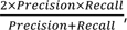, where Precision = True Positives / All Positives, and Recall = True Positives / (True Positives + False Negatives).

¹³  The chunk size should reflect research objectives, eg in our case, to differentiate topics roughly corresponding to paragraphs. While a 100-word chunk is standard, this can vary with applications.

¹⁴  Chunk embeddings can also be obtained through proprietary API services, eg as offered by OpenAI.

¹⁵  We employ a hierarchical density-based clustering method (HDBSCAN) for clustering. It groups similar items by finding densely packed areas in the data, forming clusters within clusters to reveal patterns at different levels of detail.

¹⁶  LDA is a Bayesian model that identifies topics within a text corpus by assuming that documents are mixtures of topics and that topics are mixtures of words. Each document is represented as a mixture of topics, with each word assigned to a particular topic.

¹⁷  It is possible to minimise the number of topics directly from BERTopic. However, starting with more detailed topics from BERTopic, and then using LDA to consolidate them later in a modular way, offers better control over the process and provides greater transparency and clarity for the analysis.

¹⁸  Although BERT-based models are often suitable for sentiment classification tasks, two key factors motivated our choice of a GPT-based model. First, the length of each chunk (100 words) makes the classification task more complex, requiring a high-performance model. Second, topic modelling has reduced the number of articles to a size that is feasible for processing by a large model.

¹⁹  For example, the prompt for fundamentals includes "Assign a sentiment score of –1 for negative, 0 for neutral, or 1 for positive. A positive sentiment means earnings or their outlook are upbeat, GDP growth prospects are bright, labour market remains tight [-]. A negative sentiment is the opposite [-]. Neutral sentiment is when the fundamental developments have no clear implications [-]."

²⁰  See BIS Quarterly Review (March 2024) for example.