Tools for managing banking distress: historical experience and lessons for today
We analyse the effectiveness of policy tools for large-scale banking distress and draw lessons for today. The depth of recessions following banking distress depends both on the speed with which tools were deployed and their type and on the macro-financial vulnerabilities. While, in general, swifter and broader-ranging policy actions mitigate such recessions, central banks' asset purchases and lending are particularly effective when banks have been underperforming or when distress follows abnormally large asset price movements, such as those triggered by the Covid19 crisis. Our analysis confirms that the recently employed policies have supported the real economy.1
JEL classification: G01, G38, E60.
Banking distress and crises tend to be followed by deep recessions. The basic reason is the sharp contraction in lending following a breakdown in financial intermediation. Baron et al (2020) document that after episodes of large bank stock price declines and an abnormal number of bank failures - that is, after distress episodes - real GDP falls by 5.5% on average from peak to trough. Output losses are particularly large when distress morphs into a full-scale banking crisis (Laeven and Valencia (2013)). And they vary across countries. For example, during the Great Financial Crisis (GFC) output fell from peak to trough by 0.16% in Switzerland and by almost 30% in Greece.
There are two interrelated sets of explanations for such variations across countries and episodes. One relates to the initial economic conditions, notably the macro-financial imbalances with which countries enter a period of distress. For instance, banking distress associated with the unravelling of a domestic financial imbalance (eg a housing bubble) may have a very different impact than that stemming from an external event in the absence of such or similar imbalances (eg a crisis imported through cross-border exposures).2 The other set of explanations relates to the policies employed. The timing and degree of policy activity and the specific tools deployed (eg central bank lending, separation of impaired assets) differ considerably across episodes. These choices will influence the severity of the recession, not least if the effectiveness of tools varies with the initial conditions.
Key takeaways
- Policy interventions that address banking distress also help support GDP growth.
- Central banks' asset purchases and lending have generally been effective in supporting growth when distress follows banks' poor performance, high private sector leverage or large asset price corrections.
- Central banks' swift response to the Covid-19 crisis has helped to support the economy, including by pre-emptively staving off banking distress.
While many studies document the economic consequences of banking distress, relatively few systematic cross-country analyses explore the effectiveness of mitigating policy tools.3 Progress has been hamstrung by a lack of comprehensive data about these tools. Furthermore, it is inherently difficult to measure effectiveness. For example, larger-scale distress calls for stronger interventions, but also makes success less certain. This may lead to the spurious conclusion that interventions are less effective.
With this special feature, we make progress along three dimensions. First, we classify 62 banking distress episodes into five categories, on the basis of initial macro-financial vulnerabilities.4 Second, using a new database by Adler and Boissay (2020) on the deployment of various distress mitigation tools, we assess empirically whether variations in the evolution of GDP across similar episodes can be explained by differences in the speed and type of policy interventions. Third, we draw policy lessons for today from our analysis.
We find that swifter and broader-ranging policy actions mitigate the impact of banking distress on economic activity. We refine this result in several ways. Central bank lending schemes are more effective in helping restore GDP growth when set up in the first year of distress, whereas impaired asset segregation schemes are more successful when used in the second. Asset purchase and - to a lesser degree - liability guarantee schemes are effective regardless of when they are deployed.
Our analysis of past experiences also suggests that certain tools are particularly effective under specific initial conditions. For example, we find that central bank lending schemes are most helpful when distress follows unusually large asset price corrections of the type triggered by the Covid-19 crisis. Our results confirm that the policy measures adopted since March 2020 have helped to support the economy, including by pre-emptively staving off banking distress.
The rest of this feature is structured as follows. The first section describes how we classify banking distress episodes and, in the process, documents their variety. The second describes the various policy interventions, and includes a box on their variation by time of use and across countries. The third section formally tests the effectiveness of various policy interventions depending on their speed and the type of episode. The fourth section applies these findings to the ongoing Covid-19 crisis. A final section concludes.
Classifying banking distress episodes
Banking distress has various causes and can start from different initial conditions. Such differences must be accounted for when evaluating the effectiveness of policy interventions. Our approach consists of classifying past distress episodes into categories, based on the macro-financial vulnerabilities that preceded them.
We consider 62 past banking distress episodes from Baron et al (2020) for 29 countries over the period 1980-2016.5 Baron et al define a distress episode as one in which bank equity prices fall by 30% year on year and there is a higher than normal number of bank failures. Their list differs from others' (eg Laeven and Valencia (2012, 2018)) in two ways. First, it features more episodes, including many distress episodes that did not end in crisis.6 Second, the starting dates of the episodes are identified precisely by crashes in bank stock prices.
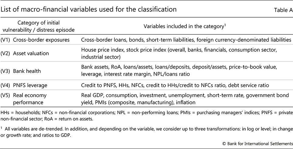
In order to classify banking distress episodes, we track the evolution of a large set of macro-financial variables in the run-up to these episodes. There are vulnerabilities when (some of) these variables take on abnormal values (Box A). We classify the episodes into five categories, corresponding to five broad vulnerability types: (V1) cross-border exposures; (V2) asset valuations; (V3) bank health; (V4) private non-financial sector (PNFS) leverage; and (V5) real economy performance (Graph 1, Box A and Adler and Boissay (2020)). Vulnerabilities of the first type, for example, typically stem from domestic residents' cross-border liabilities in foreign currencies and cross-border bank loans (Graph 1, left-hand panel). Those related to asset valuations show up as sharp drops in house and stock prices (eg following the bust of an asset price bubble). Vulnerabilities related to real economy performance manifest themselves most often through a prior severe recession, with pronounced falls in manufacturing PMIs and consumption growth.
Our classification highlights the variety of banking distress episodes. The right-hand panel of Graph 1 shows that in about 40% of the episodes, distress is preceded by excessive cross-border exposure, severe asset price corrections7 or weak real economy performance. Weak bank performance only precedes 20% of the episodes.8
Box A
Definition of vulnerabilities and classification of distress episodes
This box describes how we identify the macro-financial vulnerabilities that manifest themselves in the run-up to banking distress episodes. We say that there is a (country-specific) vulnerability whenever a variable takes on an "abnormally" high or low value, ie when it falls in the upper or lower 10% tail of its distribution. Since the immediate lead-up and aftermath of the episode may distort the statistics, we follow Goldstein et al (2000) and consider the distribution only for "normal times", defined as the period that excludes the two years before and after the beginning of distress episodes. We then investigate which variables took on abnormal values in the distress episode's starting quarter (ie of the banks' stock price crash), as well as the first, third and fifth quarters before that.
We consider a comprehensive quarterly data set of more than 70 macro-financial variables (in levels, growth rates, ratios to GDP) that the literature has identified as potential early warning indicators of banking distress (Table A). We group these variables into five categories relating to different types of macro-financial vulnerabilities. This classification follows common practice and is consistent with central banks' financial stability monitoring frameworks.
 Altogether, taking into account the number of variables and quarters considered, the total number of potential vulnerabilities per category ranges from 48 to 72, depending on the category.
To classify a distress episode, we first calculate the percentage of "abnormal" variables within a category. Then we classify an episode into a specific category if this percentage is above a threshold of 25%. The classification is not mutually exclusive: a given distress episode may be classified in multiple categories. At the same time, the 25% threshold implies that three quarters of the episodes are classified in at least one category and one quarter of all episodes are classified as not preceded by any vulnerability.
We experimented with different quarters up to the eighth quarter before the start of banking distress episodes, and our results did not change materially. See eg Borio and Lowe (2002), Borio and Drehmann (2009) and Aldasoro et al (2018). For example, in its Financial Stability Report the US Federal Reserve Board emphasises four broad categories of vulnerability: valuation pressures; borrowing by businesses and households; leverage within the financial sector; and financial institutions' funding risks (FRB (2020)). Similarly, in its Financial Stability Review the ECB focuses on: macro-financial imbalances relating to the real economic outlook; leverage in the household and corporate sectors; financial market liquidity and asset valuations; and banks' financial health (ECB (2020)). To reflect relevance, we weigh each vulnerability by how often it occurred before the distress episodes of Baron et al (2020)). For more details, see Adler and Boissay (2020).
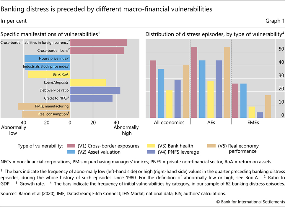
The data indicate some differences between advanced and emerging market economies (EMEs). In advanced economies (AEs), distress episodes tend to be preceded by widespread vulnerabilities, with notably excessive cross-border exposure and weak economic performance (55% of cases). In about 40% of the AE episodes, the initial conditions involve severe asset price corrections or high private sector leverage. In EMEs, it is harder to relate distress episodes to specific vulnerabilities. Just one in four episodes is preceded by excess cross-border exposure or a severe fall in asset prices, and few episodes by excess leverage, whether in the financial or non-financial sector. This suggests that banking distress in EMEs need not be the outcome of domestic imbalances, but could be triggered by external shocks.9
General patterns of policy interventions
For data on policy interventions, we draw on a new database on banking distress mitigation tools (Adler and Boissay (2020)). It contains information on more than 300 policy interventions deployed in 29 countries between 1980 and 2016. We divide policy tools into four broad types: (T1) central banks' lending schemes; (T2) bank liability guarantee schemes; (T3) impaired asset segregation (IAS) schemes; and (T4) bond and other asset purchase schemes (Box B). One advantage of the database is that it records interventions at their precise date (ie quarter) of implementation.10 Combining the databases of Baron et al (2020) and Adler and Boissay (2020) allows us to measure the lag between the beginning of a distress episode (ie when banks' stock prices crash) and specific policy interventions. This, in turn, allows us to evaluate whether the specific timing of a tool has different effects.11
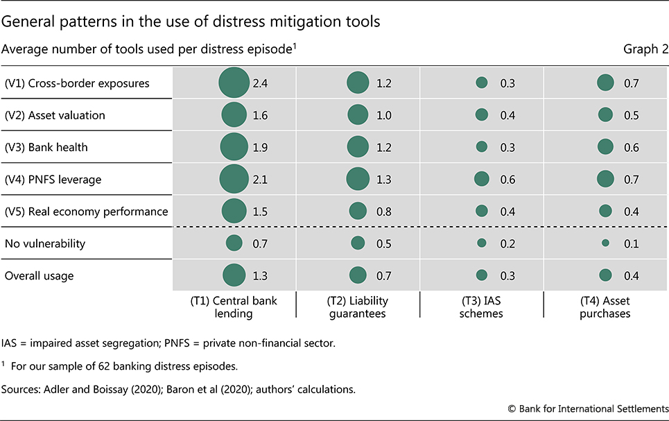
A few general patterns emerge from the combination of the two databases. For each category of initial vulnerability (rows), Graph 2 shows the average number of tools of a specific type (columns) employed in the first two years of the banking distress episodes. Overall, central banks' lending schemes are used most often, followed by bank liability guarantees, asset purchases and IAS schemes. Policy interventions mostly take place in episodes associated with at least one macro-financial vulnerability (compare the row "No vulnerability" with the other rows). Relatedly, lending schemes and asset purchases are used the most in episodes associated with cross-border border vulnerability and high private sector leverage.
Box B
A database on banking distress mitigation tools
Frederic Boissay, Stijn Claessens and Alan Villegas
This box describes Adler and Boissay's (2020) new database on banking distress mitigation tools. The database contains information on more than 300 interventions in 29 countries between 1980 and 2016. It documents the tools' deployment dates (quarter) and key design features. The tools are divided into four broad types of schemes: (T1) central bank lending; (T2) bank liability guarantees; (T3) impaired asset segregation; and (T4) asset purchases.
Central bank lending schemes (T1) consist of interventions providing funding directly to banks and other financial intermediaries. These include outright liquidity provision, special (eg long-term) lending and changes in central banks' collateral eligibility rules (eg extension of collateral frameworks to more institutions or asset classes). Among these tools, the last one is the most frequently employed.
Bank liability guarantee schemes (T2) consist of fiscal authorities (partly) guaranteeing commercial banks' privately issued debts, sometimes in exchange for a guarantee fee. An example is an enhancement to an existing deposit insurance scheme. Most schemes are optional, and cover a relatively large array of debt instruments (eg senior debt instruments, interbank debts), but are restricted to newly issued (as opposed to legacy) liabilities.
The database records 40 impaired asset segregation schemes, (T3) or so-called "bad banks". Most bad banks in the database have a limited lifetime. About half are set up for one specific bank. The other half are "centralised", ie they purchase assets on a voluntary basis from several banks, often with a limit on the amount purchased per bank. On average, the size of a bad bank amounts to 7% of GDP, and a haircut of 25% is applied on the assets purchased.
Asset purchase schemes (T4) consist of interventions where the central bank purchases specific assets on secondary markets (eg corporate bonds, asset-backed securities), or offers to banks to swap risky for safer assets (typically government bonds).
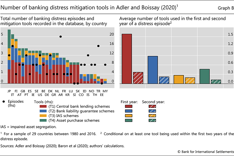
The intensity of interventions varies by country. Graph B (left-hand panel) shows that Japan, Italy and Finland record the most interventions overall. Finland has the most interventions per distress episode. When they take place, most interventions occur in the first year (right-hand panel). Central banks' lending schemes are the most prevalent type of intervention, with an average of 1.6 schemes set up in the first year, followed by bank liability guarantee schemes.
The views expressed are those of the authors and do not necessarily reflect those of the Bank for International Settlements
Assessing the effectiveness of policy interventions
Our approach to evaluating empirically the effectiveness of policy interventions involves two steps. First, we seek to establish a causal relationship between the number of tools deployed and cumulative GDP growth throughout the distress episode.12 Second, we test whether the various tools are more effective when deployed more swiftly or in particular types of distress episodes.
Further reading
Baseline econometric model
Establishing a causal relationship between a given policy intervention and GDP growth is challenging. To keep "all else" equal, we focus on banking distress episodes that feature observationally similar initial macro-financial vulnerabilities. Our identification strategy rests on the assumption that similar vulnerabilities are the symptoms of similar underlying factors, and that the latter should have similar economic consequences unless they are addressed with different policies.13
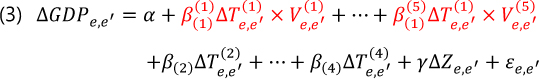
Accordingly, the unit of analysis is a pair of similar episodes e and e',14 and we are interested in whether the difference in the evolution of GDP throughout these episodes can be explained by differences in policy interventions. Our baseline econometric model is the following:

The variable ∆GDPe,e' is the difference in average annualised real GDP growth rates between episodes e and e'. To gauge post-crisis performance, we focus on GDP growth from two years before to three years after the episode starts.15 Since different policy interventions often come together in a distress episode, we estimate the effects of the four types of distress mitigation tools simultaneously. Accordingly, variables  ...,
..., are the differences between the number of tools of type (T1), ..., (T4) deployed within the first two years of episode e versus episode e'. Of interest are the coefficients β(1), ...,β(4), which capture the effect of the corresponding tools on GDP growth. The regression features a set of additional control variables ∆Ze,e' that account for drivers of GDP growth other than policy interventions. The controls notably include 0/1 dummies capturing differences between countries in terms of monetary policy rates, exchange rate regimes and central bank independence.16
Results for general effectiveness and timing
The analysis points to differences in the tools' effectiveness. The estimates of the coefficients β in regression (1) are reported in Graph 3 (left-hand panel). We find that central banks' lending schemes and asset purchases have a statistically significant positive effect on post-crisis GDP growth. In particular, every additional asset purchase scheme augments the annualised GDP growth rate by 0.5 percentage points on average.17 Additional bank liability guarantees also have a statistically significant positive effect, but marginally so. One reason could be that calibrating liability guarantee schemes (guarantee fee, requirements for participation, scope of the scheme) is challenging, and schemes may not initially be attractive to banks.18
Overall, our results are consistent with those using richer, micro data sets. Despite the usual limitations inherent to cross-country analyses employing coarse data, our findings concur with those of more granular case studies. For example, Eser and Schwaab (2016) and Andrade et al (2016) find that asset purchase schemes improve liquidity conditions, reduce risk premia and contribute to raising the equity price of the banks holding the assets covered by the scheme. Andrade et al (2019) also find that, when central banks provide long-term liquidity to banks, the latter increase their loans to the real economy. And Laeven and Valencia (2008) find that extending blanket guarantees reduces banks' need for liquidity support from central banks.
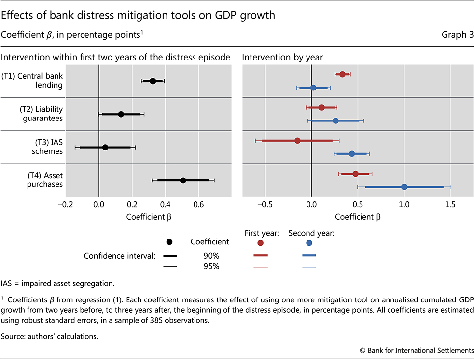
The effectiveness of policy interventions varies depending on the phase of the distress episode (Graph 3, right-hand panel). This result is obtained from a richer version of regression (1) distinguishing between tools deployed in the first or second year of the distress episode. We find that liquidity provision by central banks is effective in the first year, reflecting its stabilisation role, but not in the second, when solvency issues tend to be more prominent. In contrast, impaired asset segregation is more effective in the second year, as non-performing assets are being recognised (Ari et al (2019)) and bank balance sheets must be repaired. Asset purchase schemes are effective whenever they are deployed, but more so in the second year.19 Liability guarantees are the only exception, equally effective in the first or the second year.
Results for effectiveness by type of tool and category of banking distress
To test whether the effect of policy activity - defined as the number of tools deployed - varies with the category of distress episodes, we next estimate the following modification of regression (1):

We interact the difference in the total number of tools deployed, denoted ∆Te,e', with dummy variables  ...,
...,  , equal to one if episodes e and e' 's initial vulnerabilities both belong to categories (V1), ..., or (V5). Accordingly, the coefficient β measures the effect of deploying one additional tool (of any type) during a distress episode that is preceded by a particular macro-financial vulnerability.
The results of estimating regression (2) are reported in the left-hand panel of Graph 4. All coefficients are statistically positive and of similar size at around 0.06. This means that using altogether more of the various available tools helps address banking distress.
Next, we examine whether the effectiveness of individual tools depends on the category of initial vulnerability. To this end, we modify regression (2) by interacting a given tool with each macro-financial vulnerability:
Of interest in regression (3) are the coefficients  , ...,
 , which capture the effects of deploying a tool of type (T1) during a distress episode preceded by macro-financial vulnerability of category (V1), ..., or (V5). We estimate this model separately for each type of tool and obtain 20 (four tools times five vulnerabilities) distinct estimates. The right-hand panel of Graph 4 shows the effect on GDP growth (in percentage points) of deploying a given tool (columns) in a given type of distress (rows). The size of a dot reflects the size of the effect, and a green dot indicates that the effect is statistically significant.
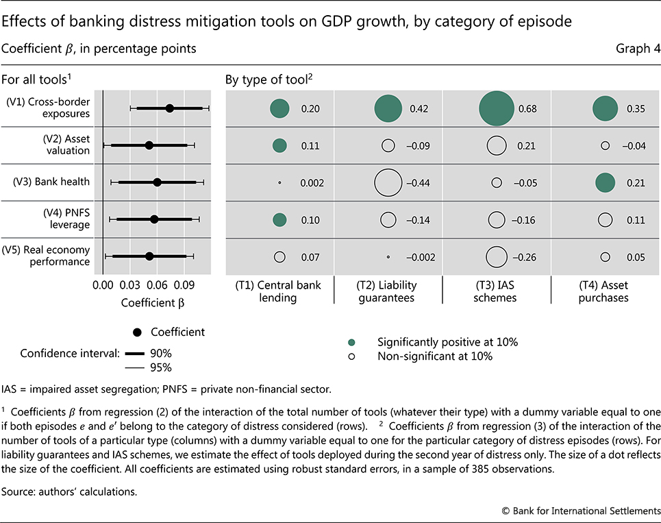
While using more tools is beneficial regardless of specific initial conditions (Graph 4, left-hand panel), certain tools are especially effective under specific initial conditions (right-hand panel). For instance, we find that more lending schemes and asset purchases boost GDP growth - by 0.2 percentage points and 0.35 percentage points, respectively - when distress follows abnormally large cross-border exposure. Likewise, such interventions are effective on the heels of large asset price corrections, weak bank performance and excess private sector leverage. From the perspective of specific vulnerabilities, we find that all tools - and, especially, impaired asset segregation schemes - are effective in a context of excessive cross-border exposure. In contrast, no single tool is especially potent when a country enters a banking distress episode with weak economic performance. This could reflect the lack of direct central bank levers to address distress that originates in the real economy.20 There are nonetheless complementarities between tools in the case of weak economic performance, because deploying multiple tools concomitantly helps to address distress (left-hand panel, last row).21
Insights for today
The Covid-19 economic shock is the largest and most singular global shock experienced in modern peacetime. It was triggered by a global pandemic and synchronised lockdowns, which resulted in inability to work, disruptions in global supply chains and an abrupt fall in aggregate demand, leading to a severe recession.
The financial sector has also been stressed by the shock. In many countries, banks' stock prices plummeted in the first quarter of 2020, even more so than those of other firms (Graph 5, left-hand panel), and are still well below their pre-crisis levels (Aldasoro et al (2020)). In some countries, the equity price drop was more than 30%, one of the two conditions for banking distress in Baron et al (2020).22
The fall in bank equity prices came on the back of overall relatively benign macro-financial conditions. Compared with past banking distress episodes, few countries entered the Covid-19 crisis with significant macro-financial vulnerabilities (Graph 5, centre panel: compare filled with unfilled bars). As of Q1 2020, the most frequent vulnerabilities related to asset valuations and PNFS leverage. Even these showed up, respectively, in only 10% and 5% of the countries (plain bars)23 and only 20% and 10% of the countries where banks' stock prices fell by more than 30% (striped bars).
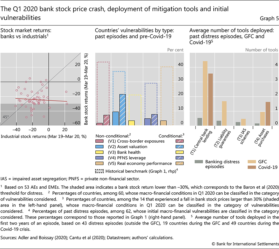
Central banks have responded swiftly and forcefully to the Covid-19 shock, with many interventions similar to those analysed in this special feature - notably targeted lending operations and asset purchases.24 Responses so far closely match in number those taken during the GFC, and are substantially more than those in previous banking distress episodes (Graph 5, right-hand panel).
These interventions have helped banks remain resilient and support economic sectors affected adversely by the crisis. Lessons from our historical analysis underscore the benefits of a swift deployment of central banks' toolbox (see also CGFS (2019)). They also underscore that, in episodes preceded by bank underperformance or featuring abnormally large asset price corrections, central banks' targeted lending and asset purchases are particularly effective. As all this matches salient characteristics of the Covid-19 crisis and the attendant policy interventions, our analysis confirms that these interventions have helped to stave off banking distress and support growth.
Conclusion
The effectiveness of banking distress mitigation tools depends on both the speed and type of tools employed and the preceding financial and economic vulnerabilities. We find that greater and swifter overall policy activity reduces the adverse impact of banking distress on economic activity regardless of vulnerabilities. Central bank lending and asset purchase schemes are most effective in helping restore GDP growth in times of banking distress that follow low asset valuations, high bank leverage and weak bank performance.
Our analysis comes with many of the usual caveats. First, due to data limitations, we proxy policy intervention intensity by the number of tools used - not their size - and we do not capture all the institutional and other country differences that may affect economic outcomes. Second, we measure the effectiveness of policy interventions based on their short-term impact (within two years) on GDP growth. We ignore longer-term aspects, such as the potential effects on resource allocations, moral hazard or public finances, though the latter are an important consideration as public balance sheets are currently stretched in many economies.
Triggered by a global pandemic and synchronised lockdowns, the current recession greatly differs from those that typically follow banking crises. Still, bank valuations are under pressure, reflecting financial markets' stress and the effects of the recession. Our analysis suggests that central banks' swift response to the Covid19 crisis, especially their large-scale lending and asset purchases, has helped - as in other instances - to stave off banking distress. Together with the regulatory capital and liquidity buffers built over the past decade, these policy interventions have helped banks weather the shock and be a source of stability, supporting the economy.
References
Adler, K and F Boissay (2020): "Dealing with bank distress: insights from a comprehensive database", BIS Working Papers, forthcoming.
Aldasoro, I, C Borio and M Drehmann (2018): "Early warning indicators of banking crises: expanding the family", BIS Quarterly Review, March, pp 29-45.
Aldasoro, I, I Fender, B Hardy and N Tarashev (2020): "Effects of Covid-19 on the banking sector: the market's assessment", BIS Bulletin, no 12, May.
Andrade, P, J Breckenfelder, F De Fiore, P Karadi and O Tristani (2016): "The ECB's asset purchase programme: An early assessment", ECB Discussion Paper, no 1956.
Andrade, P, C Cahn, H Fraisse and J-S Mésonnier (2019): "Can the provision of long-term liquidity help to avoid a credit crunch? Evidence from the Eurosystem's 3-year LTROs", Journal of the European Economic Association, vol 17, no 4.
Ari, A, S Chen and L Ratnovski (2019): "The dynamics of non-performing loans during banking crises: a new database", IMF Working Papers, no WP/19/272.
Baron, M, E Verner and W Xiong (2020): "Banking crises without panics", Quarterly Journal of Economics, forthcoming.
Basten, M, E Bengtsson, B Klaus, A Koban, P Kusmierczyk. J-H Lang and M Lo-Duca (2017): "A new database for financial crises in European countries: ECB/ESRB EU crises database", ECB Occasional Papers, no 194.
Boar, C, L Gambacorta, G Lombardo and L Awazu Pereira da Silva (2017): "What are the effects of macroprudential policies on macroeconomic performance?", BIS Quarterly Review, September, pp 71-88.
Borio, C and M Drehmann (2009): "Assessing the risk of banking crises - revisited", BIS Quarterly Review, March, pp 29-46.
Borio, C and P Lowe (2002): "Assessing the risk of banking crises", BIS Quarterly Review, December, pp 43-54.
Borio, C, B Vale and G von Peter (2010): "Resolving the financial crisis: are we heeding the lessons from the Nordics?", BIS Working Papers, no 311, June.
Cantu, C, P Cavallino, F De Fiore and J Yetman (2020): "A global database on central banks' response to Covid-19", BIS Working Papers, forthcoming.
Cecchetti, S, M Kohler and C Upper (2009): "Financial crises and economic activity", NBER Working Papers, no 15379.
Cerutti, E, S Claessens and L Laeven (2017): "The use and effectiveness of macroprudential policies: New evidence", Journal of Financial Stability, vol 28.
Claessens, S, D Klingebiel and L Laeven (2003): "Financial restructuring in banking and corporate sector crises: what policies to pursue?", in M Dooley and J Frankel (eds), Managing currency crises in emerging markets, University of Chicago Press,pp 147-80.
----- (2005): "Crisis resolution, policies, and institutions: empirical evidence", in P Honohan and L Laeven (eds), Systemic financial crises: containment and resolution, Cambridge University Press, pp 169-94.
Claessens, S, A Kose, L Laeven and F Valencia (2014): Financial crises: causes, consequences, and policy responses, International Monetary Fund.
Committee on the Global Financial System (2019): "Unconventional monetary policy tools: a cross-country analysis", CGFS Papers, no 63.
Detragiache, E and G Ho (2010): "Responding to banking crises: lessons from cross-country evidence", IMF Working Paper, no 10/18.
Eser, F and B Schwaab (2016): "Evaluating the impact of unconventional monetary policy measures: Empirical evidence from the ECB's Securities Markets Programme", Journal of Financial Economics, vol 119, no 1.
European Central Bank (2020): Financial Stability Review, May.
Federal Reserve Board (2020): Financial Stability Report, May.
Goldstein, M, G Kaminsky and C Reinhart (2000): "Assessing financial vulnerability: an early warning system for emerging markets", Foreign Affairs, vol 79.
Laeven, L and F Valencia (2008): "The use of blanket guarantees in banking crises", IMF Working Paper, no 08/250.
----- (2012): "Systemic banking crises: an update", IMF Working Paper, no 12/163.
----- (2013): "The real effects of financial sector interventions during crises", Journal of Money, Credit and Banking, vol 45, no 1.
----- (2018): "Systemic banking crises revisited", IMF Working Paper, no 18/206.
1 The authors thank Iñaki Aldasoro, Claudio Borio, Benoît Mojon, Vasily Pozdyshev, Hyun Song Shin, Nikola Tarashev and Christian Upper for helpful comments. The views expressed in this article are those of the authors and do not necessarily reflect those of the Bank for International Settlements.
2 The different impact of the GFC in Greece and Switzerland is a case in point.
3 In addition to country-specific case studies, the cross-country studies exploring the effects of crisis mitigation tools include Borio et al (2010), Cecchetti et al (2009), Claessens et al (2003, 2005), Detragiache and Ho (2010) and Laeven and Valencia (2013). For a general review of financial crises, see Claessens et al (2014).
4 We use Baron et al's (2020) list of banking distress episodes for 29 countries since 1980.
5 Baron et al's (2020) list includes distress episodes for more countries over the period 1870-2016, but throughout this special feature we only consider those countries and years for which we also have information on policy interventions. These countries are: Argentina, Austria, Belgium, Colombia, Denmark, Estonia, Finland, France, Germany, Greece, Iceland, Indonesia, Ireland, Italy, Japan, Korea, Luxembourg, Malaysia, the Netherlands, Norway, Portugal, Slovakia, Slovenia, Spain, Sweden, Thailand, Turkey, the United Kingdom and the United States, with emerging market economies in italics.
6 Baron et al (2020) contains about 50% more episodes than Laeven and Valencia (2018) for the same countries.
7 These are price corrections other than of bank equity prices (which are part of Baron et al's (2020) definition of bank distress), such as those of non-financial corporations' equity prices and house prices.
8 Episodes may not overlap. About one quarter of episodes feature only one type of vulnerability, and one quarter feature at least three types simultaneously. Most of the latter correspond to the GFC.
9 This can also reflect the lack of data (notably cross-border borrowing data) before EMEs' distress episodes.
10 Dates correspond to the actual implementation of the schemes, not to their announcement.
11 A limitation of the Adler and Boissay (2020) database is that it does not contain information on the size of the policy interventions. Data on the size of banking distress mitigation schemes are often not available. And even when they are, many issues prevent comparability (eg facilities of the same size may be used to different degrees, with liability guarantees and liquidity facilities being cases in point). Similar caveats apply to studies on the effects of macroprudential tools (eg Boar et al (2017), Cerutti et al (2017)). All countries covered in Adler and Boissay (2020) are in the Baron et al (2020) database except Estonia, for which we use the bank distress episodes reported in Basten et al (2017).
12 For a similar analysis with alternative metrics of success, see Adler and Boissay (2020).
13 Ideally, one would compare episodes that differ only in terms of the scope and timeliness of policy interventions, eg where policymakers also face similar institutional constraints and fiscal space, and not only episodes with similar initial macro-financial vulnerabilities. These and other issues are admittedly limitations to comparing like with like. For example, one cannot exclude that even observationally similar vulnerabilities have different causes, and thus may call for different policies.
14 Episodes e and e' feature the same type of initial vulnerabilities, ie both belong to at least one common category (V1), -, or (V5). For our sample of 62 distress episodes, there are 1,891 (= 62 x 61 / 2) possible distinct pairs, of which only 385 are deemed to contain similar episodes. Thus, we work with a sample of 385 observations. For more details about the pairing, see Adler and Boissay (2020).
15 We use GDP two years before the start of the episode because, closer to the start, GDP could be boosted by macro-financial imbalances. Part of the correction during a distress episode may then reflect a reversal to a normal growth path, for which policy interventions do not seek to correct.
16 A reduction in the monetary policy rate can also be seen as a banking distress mitigation tool. Here, we use it as a control variable, as our focus is on the effectiveness of other measures.
17 There are several possible transmission channels of central bank asset purchases to the real economy. One is a portfolio rebalancing channel, whereby purchases of sovereign bonds induce a decline in their yields and give investors an incentive to invest in corporate bonds, thus supporting the real economy. Another is a capital relief channel, as the higher price of sovereign bonds induced by central banks' purchases benefits banks that hold such bonds.
18 Banks may not participate if, for example, the scheme requires high regulatory capital ratios. Moreover, liability guarantee schemes can be dictated by urgency (eg a sudden depositor run), for which we do not fully control in our econometric analysis. This means their coefficient estimates could be biased downward due to reverse causality.
19 In all the cases above, the effects in the first and second year are statistically significantly different.
20 Indeed, all the tools considered here work primarily through banks and to a lesser degree through various other segments of the financial sector.
21 Unfortunately, the variation in the usage of tools is too limited and our sample too short to test explicitly for complementarities between the various tools.
22 To qualify as a banking distress episode according to Baron et al (2020), the Covid-19 crisis should also feature a higher than normal number of bank failures, which is not the case.
23 In March, non-financial stock prices fell sharply but house prices did not.
24 Fiscal authorities have responded to the economic disruptions too, with policy interventions of unprecedented scope and magnitude. Given the origin of the shock, many of these policies break new ground, notably the ample fiscal support to households and firms.