Household debt: recent developments and challenges
The responsiveness of aggregate expenditure to shocks depends on the level and interest rate sensitivity (duration) of household debt, as well as on the liquidity of the assets it finances. Household-level spending adjustments are more likely to be amplified if debt is concentrated among households with limited access to credit or with less scope for self-insurance. The way in which household indebtedness affects the sensitivity of aggregate expenditure matters for both macroeconomic and financial stability. Financial institutions can suffer balance sheet distress from both direct and indirect exposure to the household sector. From a macroeconomic stability viewpoint, monetary transmission is the key issue. In a high-debt economy, interest rate hikes could be more contractionary than cuts are expansionary. These considerations point to a complementarity between current macroprudential and future monetary policy.1
JEL classification: E21, E24, E52, E58, D15, G01.
Anna Zabai explains how high household debt could affect economic and financial stability (1.44 mins)
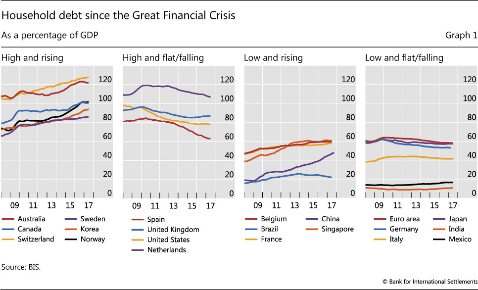
Ten years after breakdowns in housing finance markets plunged the financial system into crisis, household debt levels are again rising, with debt-to-GDP ratios reaching historical highs in several countries (Graph 1). Central banks are increasingly concerned that this may pose a threat to macroeconomic and financial stability (eg Reserve Bank of Australia (2017), Bank of Canada (2017), Bank of England (2017)).
After discussing key developments in household debt since the Great Financial Crisis (GFC), this special feature seeks to highlight some of the mechanisms through which household debt may threaten both macroeconomic and financial stability.
Debt lets households smooth shocks and invest in high-return assets such as housing or education, raising average consumption over their lifetimes. However, high household debt can make the economy more vulnerable to disruptions, potentially harming growth. As aggregate consumption and output shrink, the likelihood of systemic banking distress could increase, since banks hold both direct and indirect credit risk exposures to the household sector.
This special feature starts by discussing recent developments in household debt, focusing on trends, levels, and composition but also considering buffers and debt burdens. The following two sections discuss the implications for macroeconomic and financial stability, as sketched out above. They also provide evidence that high household debt can indeed slow economic growth in the medium term, possibly increasing the likelihood of systemic distress. A concluding section highlights some of the issues relevant for monetary and macroprudential policies.
How has household debt developed since the GFC?
Countries can be broadly classified into four groups, based on the level and trend of household debt as a ratio to GDP (debt ratio). An especially significant group comprises those countries with debt ratios that are both high (eg over 60% of GDP on average since the GFC) and trending higher (Graph 1, first panel).2 Among these, the debt ratio now exceeds 120% in both Australia and Switzerland. Countries in the second group also have high household debt relative to GDP, but the debt ratio trend seems to have either levelled off or declined in recent years (Graph 1, second panel). The two right-hand panels in Graph 1 relate to countries with average household debt ratios below 60% in the period since 2007. Among these, the third panel shows countries where debt ratios have been trending up during the past 10 years, while the fourth displays some where debt has fallen.
The composition of household debt is heavily skewed towards housing-related debt (Table 1, columns 1 and 2). Mortgages make up the lion's share of debt (between 62 and 97% in the group of countries considered here), a share that has remained broadly stable since the GFC. Households may take out mortgages to buy not only a primary residence but also properties that are rented out.3
In order to assess the implications of elevated household debt levels, it is crucial to have a sense of whether households can bear the resulting debt burdens without resorting to large adjustments in consumption should circumstances worsen.
To that end, it is important to establish whether households have been accumulating buffers that can help smooth unexpected adverse changes. The left-hand panel of Graph 2 reports household "leverage", defined here as the ratio of household debt to financial assets. Leverage is flat for countries in the first and third groups from Graph 1, suggesting that households in countries with rising debt have also seen the value and amount of their assets rise. Households in the second group, where debt is high but falling, seem to have made the most significant progress in repairing balance sheets, with leverage dropping more than 10 percentage points in the 10 years since the GFC.
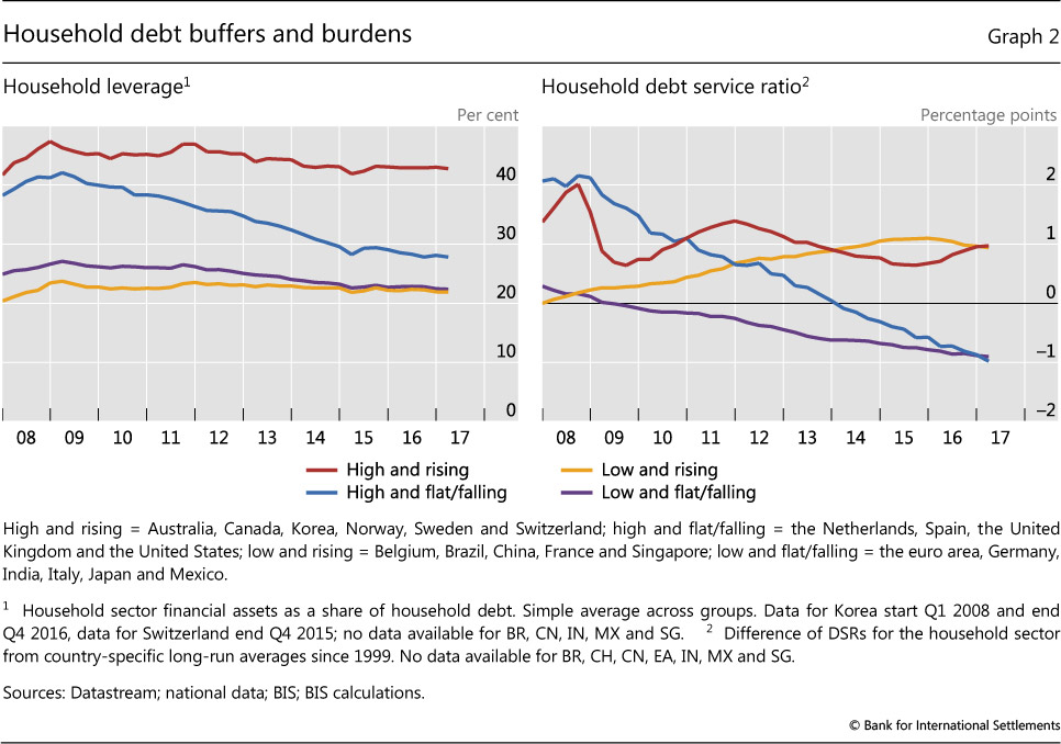
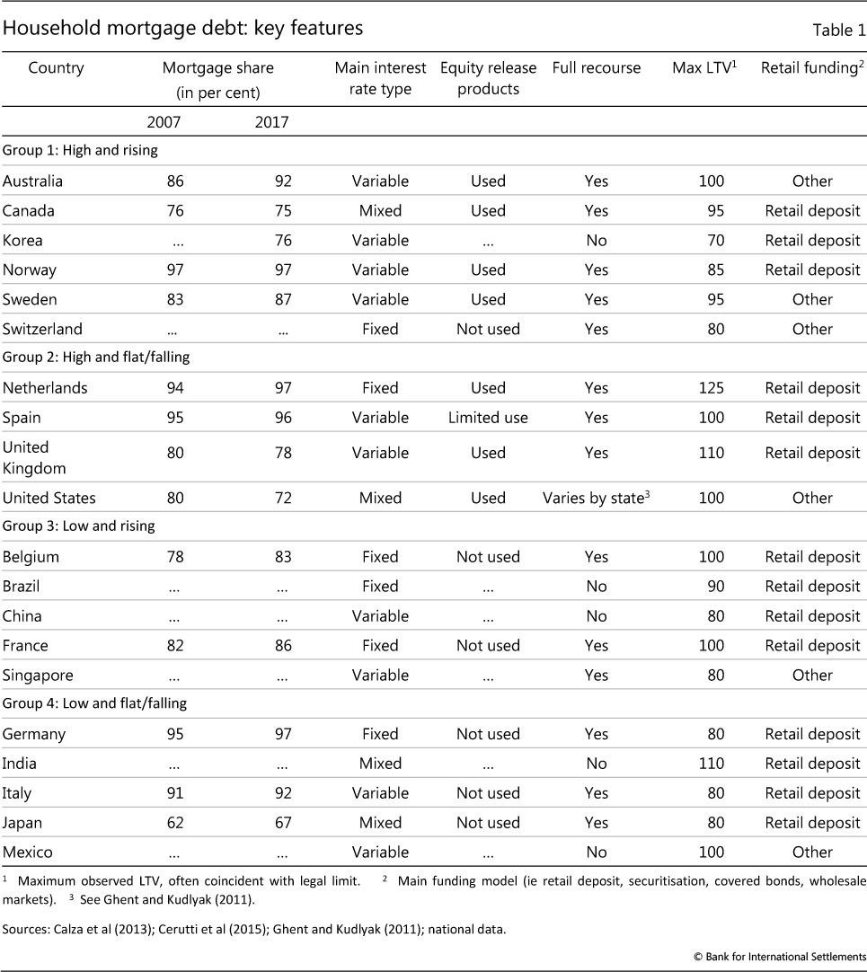
The size of household debt burdens matters too. This is best measured by the ratio of interest payments and amortisation to income - the debt service ratio (DSR; Drehmann et al (2015)). In countries where household debt has been on the rise (groups 1 and 3), DSRs have consistently exceeded their long-term averages in the 10 years since the GFC (Graph 2, right-hand panel). The DSR dynamics, however, differ across the two groups. While the DSR has been on an upward trend in group 3, its level has been more volatile in group 1. As shown in Table 1, countries in group 1 are mostly "adjustable rate" countries, while countries in group 3 are mostly "fixed rate" (column 3). This observation suggests that, while DSRs in the latter group have been pushed up by credit growth, falling interest rates have played a bigger role in the former group, occasionally offsetting the effect of higher credit on debt service burdens.4 In countries where household debt has been flat or falling (groups 2 and 4), by contrast, the DSR has been trending down since 2007.
Household debt and the economy
The level and distribution of household debt affects the responsiveness of aggregate demand and aggregate supply in the wider economy to shocks. In turn, this has implications for macroeconomic and financial stability.
Household debt and macroeconomic stability
A household's stock of debt affects its ability to deal with an unanticipated deterioration in its circumstances, such as lower income, lower asset prices or higher interest rates. In order to avoid cutting consumption too much, the household has a number of options. First, it can draw down savings. Assets such as current account balances, stocks or mutual funds can easily be converted into cash. By contrast, illiquid assets such as housing can be pledged for borrowing only in jurisdictions where equity release products such as home equity lines are available (Table 1, column 4). In this sense, assets can work as self-insurance. Formal insurance options, whether private or public (eg unemployment insurance), may also be on hand. Second, the household can adjust its debt. It can try to reduce its existing debt burden by renegotiating or refinancing. In jurisdictions where loans are not full-recourse (Table 1, column 5), it could also default strategically. And if it retains access to markets, it could obtain additional (unsecured) credit.
Several features of a household's indebtedness will influence the attractiveness of these options and hence the ultimate cut in consumption.5 First, a highly levered household is less likely to be able to adjust by borrowing, as lenders would be less forthcoming. These households are said to be closer to their "borrowing constraints". Mortgage lenders, for example, typically impose loan-to-value ceilings on new loans (Table 1, column 6). Indeed, there is evidence that, after the GFC, households with higher debt- to-income ratios - a proxy for leverage - cut spending by more than those with lower ratios. Between 2007 and 2009, spending cuts by UK households with debt ratios above 400% were 10 times higher than those of households with ratios below 100% (Bunn and Rostom (2015)). In Norway the difference in response was somewhat less pronounced but households with low debt burdens actually increased spending (Fagereng and Halvorsen (2016), Bank of England (2017)).
Second, the more illiquid the wealth financed through debt, the higher the cut in consumption. Examples might be large shares of wealth in housing (ie mortgage debt) or human capital (ie student debt), as confirmed by Kaplan et al (2014). The behaviour of such households and individuals could be an important driver of aggregate expenditure where high debt levels coincide with a large share of wealth locked up in residential property, as in Sweden. Similarly, in Australia, the liquid pre-payment buffers on mortgage-offset accounts are heavily concentrated on older mortgages with less time to maturity.6 For one third of mortgages, available repayment buffers cover no more than one month's worth of loan payments (Reserve Bank of Australia (2017)).7
Accounting for the increase in the stock of debt: credit demand vs credit supply
Rising household debt can reflect either stronger credit demand or an increased supply of credit from lenders, or some combination of the two.
Unconstrained households can borrow in order to smooth consumption before an anticipated increase in income or after an unexpected temporary drop in income (eg illness, accidents, short-term unemployment). In addition, households borrow to finance investment in illiquid assets with high long-term returns such as housing (Kaplan et al (2014)). Credit demand might rise because households are optimistic about income prospects, or because costs (interest rates) are low. The post-Great Financial Crisis period has seen extraordinary monetary accommodation, very low borrowing rates and low returns on safe assets. This combination has lifted debt-financed demand for housing, either for own use or as an investment (eg in Germany, property has recently been referred to as "concrete gold").
Structural factors such as demographic shifts could also be playing a supporting role. Population growth could have contributed to the rise in credit in Australia and Canada. Structural factors combine with demand factors in Korea: returns on real estate investments have been especially high, encouraging households close to retirement to borrow to invest in buy-to-let properties with the aim of generating income for old age.
Favourable supply conditions can also boost credit to households. In Australia, for instance, heightened competition among lenders seems to have resulted in a relaxation of lending standards. There is some evidence that this may also matter for UK consumer credit (Bank of England (2017)). In Korea, solvency (loan-to-value ratios) and affordability (debt-to-income ratios) requirements on new loans have been relaxed as part of a broader easing of real estate regulation. In the United States, the government has supported the secondary mortgage market through its long-standing implicit guarantee of debt issued by government-sponsored enterprises. In addition, the post-crisis world has been marked by greater emphasis on a more traditional, retail-oriented approach to banking.
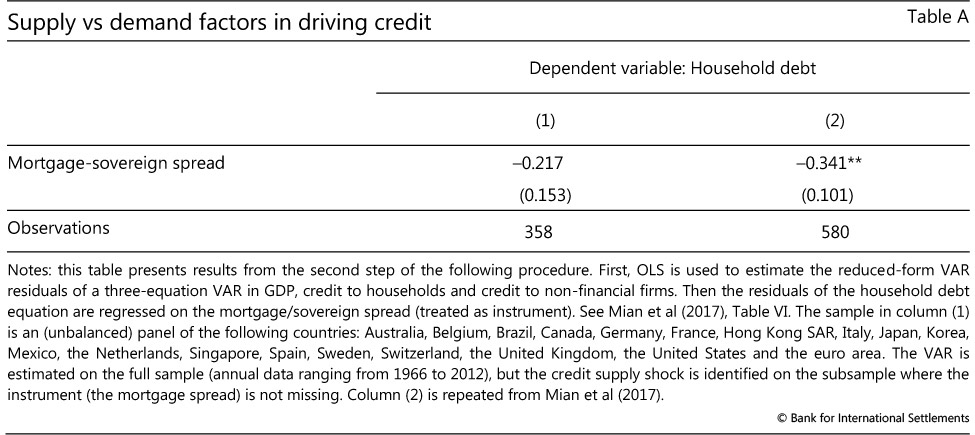
Table A presents evidence that supply factors may have been more important than demand in driving household credit in some jurisdictions. The coefficients are computed following Mian et al (2017), who estimate a proxy vector autoregression (VAR) in two steps. A negative (positive) coefficient implies that increases in credit to households that are not explained by the dynamics of GDP growth, credit to households itself and credit to non-financial firms are associated with narrow (wide) mortgage spreads, which are in turn more likely to be correlated with outward shifts in credit supply than in credit demand. The results shown in column 1 use the sample of countries listed in Table 1. These results are qualitatively consistent with the findings of Mian et al (2017), who consider a broader range of countries (column 2), although the estimates are not as precise because of the smaller sample size.
Between 2012 and 2016, the number of households in the 60+ age group owning buy-to- let properties has grown by about 50%, and accounts for most of the growth in such investments. The investments are largely debt-financed.
Third, the interest rate sensitivity of a household's debt service burden is likely to matter. The greater the interest rate sensitivity - or duration - of a household's liabilities relative to that of its assets, and the shorter the maturity of these liabilities, the larger the impact on consumption (Auclert (2017)). This effect would be bigger in countries with more debt at variable rates.
Finally, high debt (relative to assets) can make a household less mobile, and hence less able to adjust by finding a new or better job in another town or region. Homeowners may be tied down by mortgages on properties that have depreciated in value, especially those that are underwater (ie worth less than the loan balance). The trend of homeownership tenure in the United States is consistent with this possibility. The median homeownership tenure there was about four years over the period 2000-07, but it has been rising steadily since and has now approximately doubled.8
These household-level observations have implications for aggregate demand and aggregate supply. From an aggregate demand perspective, the distribution of debt across households can amplify any drop in consumption. Notable examples include high debt concentration among households with limited access to credit (ie close to borrowing constraints) or less scope for self-insurance (ie low liquid balances).
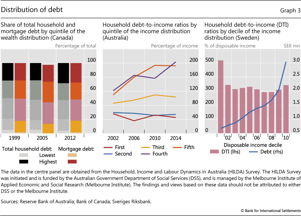
Since poorer households are more likely to face these credit and liquidity constraints, an economy's vulnerability to amplification can be assessed by looking at the distribution of debt by income and wealth. In many countries, most debt is held by households in the top quintiles of the income and wealth distribution. In Canada, for example, the two top quintiles hold approximately 50% of total and mortgage debt (Graph 3, left-hand panel). In Australia, households in the top income brackets tend to have substantially higher debt ratios than those at the bottom of the distribution (eg in 2014, the top two quintiles had debt ratios of about 200%, while the bottom two had ratios of about 50%, centre panel). This is not necessarily the case everywhere, however. In Sweden, the debt ratio is more equally distributed across the income distribution (right-hand panel).
Moreover, all else equal, one would expect the impact of indebtedness on monetary transmission to be larger in economies where household debt is high and adjustable-rate debt is more prevalent (see also Hofmann and Peersman (2017, this issue) and BIS (1995)). Monetary policy is likely to have asymmetrical effects in a high-debt economy, meaning that interest rate hikes cause aggregate expenditure to contract more than cuts would cause it to expand (Sufi (2015)). This is because credit-constrained borrowers cut consumption a lot in response to interest rate hikes, as their debt service burdens increase. However, they do not expand it as much in response to cuts of equal magnitude. They prefer to save an important fraction of their gains so as to avoid being credit-constrained again in the future (Di Maggio et al (2017)). The asymmetry is likely to increase as the duration of household liabilities shortens, as this boosts the impact of interest rate hikes on their debt service burdens.
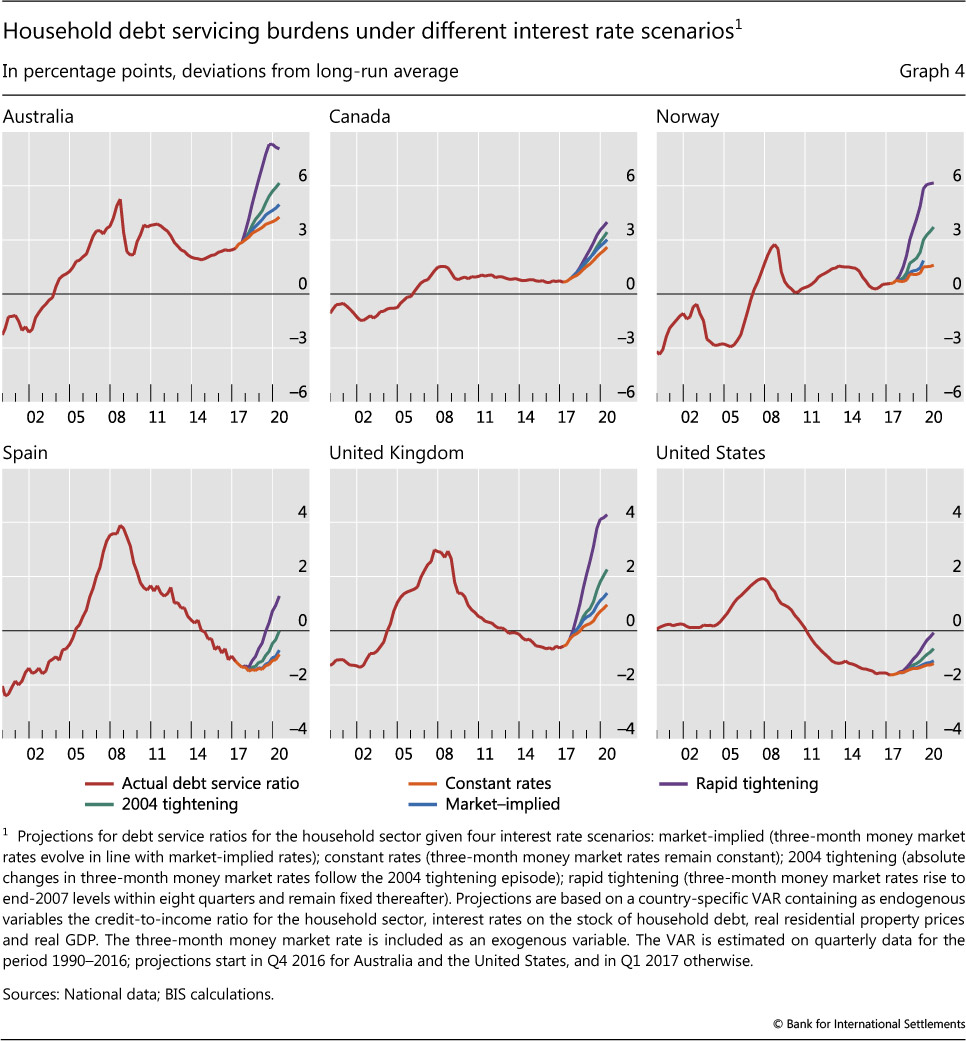
BIS simulation analysis (BIS (2017)) provides evidence consistent with the observation that DSRs are more sensitive to rate hikes in economies where the duration of household debt is shorter (Graph 4).9 In countries where household debt has risen rapidly since the crisis, and where the majority of mortgages are adjustable-rate, DSRs are already above their historical average, and would be pushed yet further away by higher interest rates (eg in group 1, Australia and Norway; see Table 1, column 3, and Graph 4, top row). By contrast, countries where households have been actively repairing their balance sheets post- crisis (eg in group 2, Spain and the United States, see Table 1, column 3, and Graph 4, bottom row) appear less vulnerable to an increase in rates, despite the large share of adjustable-rate mortgages.
From an aggregate supply perspective, an economy's ability to adjust via labour reallocation across different regions can weaken if household leverage grows over time. In such an economy, a fall in house prices - as may be associated with interest rate hikes - would saddle a number of households with mortgages worth more than the underlying property. A share of these "underwater" homeowners might also lose their jobs in the ensuing contraction. In turn, their unwillingness to realise losses by selling their property at depressed prices may prolong their spell of unemployment by preventing them from taking jobs in locations that would require a house move. As a result, the economy could experience a higher rate of structural unemployment. However, empirical evidence for this lock-in effect is mixed (eg Valletta (2013)).
Household debt and aggregate demand: some evidence
A growing body of evidence points to the existence of a "boom and bust" pattern in the relationship between household debt and GDP growth (Mian et al (2017), Lombardi et al (2017), IMF (2017)). An increase in credit predicts higher growth in the near term but lower growth in the medium term.
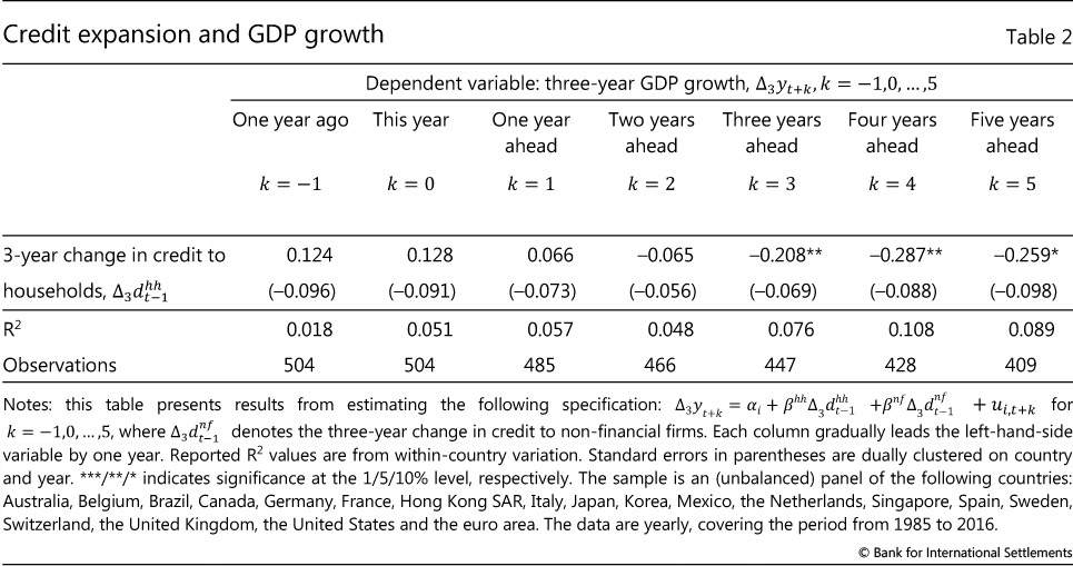
This boom-bust pattern appears to be robust across different samples. Table 2, following Mian et al (2017), takes a first stab at exploring the relationship between household debt and GDP growth by looking at correlations. The first row presents estimates of the impact of past changes in household debt on GDP growth, both contemporaneously and in subsequent periods. The first column reports the estimate of the impact of the change in household debt between year t − 4 and t − 1 (ie the three-year change in the debt level) on GDP growth in year t − 1, the second column the impact on growth in year t (ie one year ahead) and so on, until the last column, which shows the impact in t + 5 (ie five years ahead).10
The first row confirms the existence of a boom-bust pattern. Higher debt boosts growth in the near term but reduces it over a longer horizon. This impact is both economically and statistically more meaningful further into the future. The estimates reported in the first row are consistent with those of the original study, although the precision is lower due to a smaller sample size (second row, in parentheses).
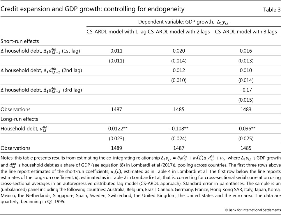
The boom-bust pattern is also robust to changes in the empirical approach. For example, Lombardi et al (2017) use a co-integrating model that can distinguish between short- and long-term effects.11 The short-term coefficients are all positive, albeit not statistically significant, while the long-term coefficients are negative and significant (Table 3).
Household debt and financial stability
Elevated levels of household debt could pose a threat to financial stability, defined here as distress among financial institutions. In most jurisdictions, this is chiefly because of sizeable bank exposures.12 These exposures relate not only to direct and indirect credit risks, but also to funding risks.
The direct exposure to credit risk associated with household debt reflects the likelihood that borrowers will default. Defaults occur when debt service costs become hard to bear because interest rates increase or incomes fall (eg in a recession). There is some evidence that this may be occurring in Australia, where high-DSR households are more likely to miss mortgage payments (Read et al (2014)).
Moreover, if higher interest rates reduce collateral values, such as house prices, (eg Aladangady (2014)), recovery values will also take a hit. In other words, banks will face a higher loss-given- default. In jurisdictions where strategic default is a possibility - because loans are less than full recourse (eg China, Brazil, India, Korea, Mexico, see column 5 in Table 1) - fire sales could depress collateral values further.
The indirect exposure to household debt arises from any increase in credit risk linked to households' expenditure cuts. These are bound to have a broader impact on output and hence on credit risk more generally. Deleveraging by highly indebted households could induce a recession so that banks' non-household loan assets are likely to suffer.13 This indirect channel is arguably more difficult to quantify, but it is probably more important in jurisdictions where households have relatively more limited access to credit markets and a capacity for self-insurance.
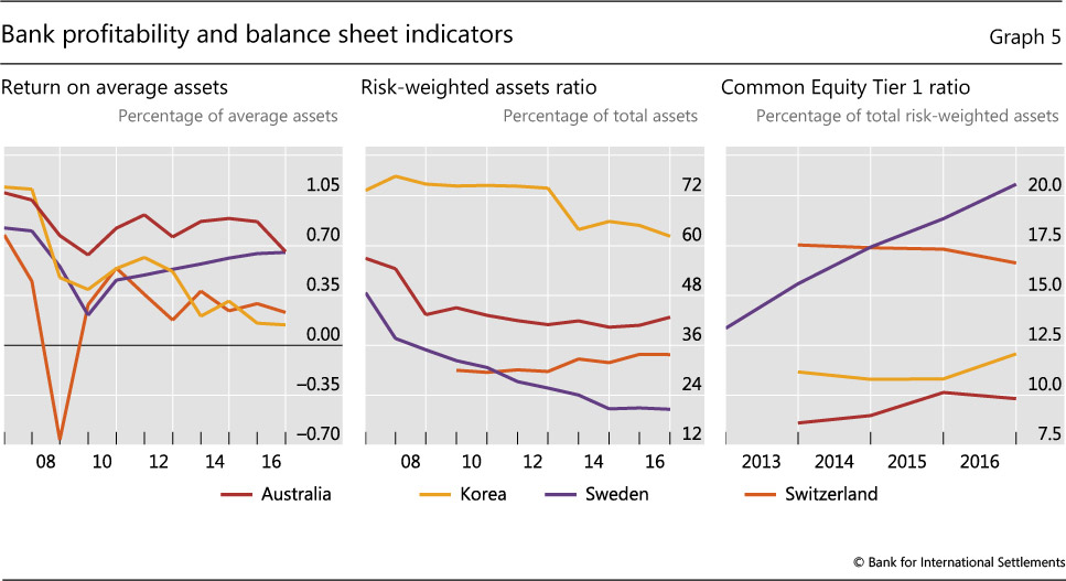
Arguments made in the previous section imply that direct and indirect risk exposures to households are positively correlated, so that mortgages are likely to perform badly just when households are cutting consumption. An important issue, then, is whether banks are equipped to deal with these risks. Bank profitability in several countries has been sluggish in the 10 years since the GFC (Graph 5, left-hand panel), limiting banks' ability to use retained earnings to cushion unexpected losses. In addition, the concurrent expansion in mortgage credit is in large part driving a decline in average risk weights - mortgages are not seen to be as risky as, eg, corporate loans - especially in Australia and Sweden (Graph 5, centre panel). Any corresponding concentration of mortgages in banks' portfolios implies that direct credit risk exposures to the household sector could deplete a large chunk of their capital buffers if mortgage performance deteriorates significantly. Moreover, this would happen at the same time as indirect credit risk exposures deteriorate, putting further strain on bank balance sheets. That said, bank capital positions are generally strong; Swedish and Swiss banks, in particular, appear to have ample capital cushions (Graph 5, right-hand panel).
Financial stability may also be threatened by funding risks (Table 1, column 7). In Sweden (as in much of the euro area), banks fund mortgages by issuing covered bonds, which are held primarily by Swedish insurance companies and other banks.14 This network of counterparty relationships could become a channel for the transmission of stress, as any decline in the value of one bank's cover pool could rapidly affect that of all the others. That said, covered bonds are dual recourse, so buyers have a claim both on the collateral pool and on the issuer. This might mitigate the risk of default and contagion. Korea has recently introduced policies to develop loan securitisation as an alternative funding source.15 Plain vanilla securitisation removes credit risk from the balance sheet of banks and transfers it to investors. To the extent that the latter are less leveraged, such a transfer may mitigate financial stability risks. However, as the GFC illustrated, securitisation poses its own risks that need to be understood and managed by investors and other counterparties.
This discussion suggests that household-based credit measures could be good predictors of systemic banking distress, much like broader credit measures (eg Borio and Lowe (2002), Drehmann and Juselius (2014), Jordà et al (2016)). Among these, the credit gap - defined as the difference between total credit to GDP and its long-term backward-looking trend - and the total DSR are of special interest. While the credit gap is typically found to be the best leading indicator of distress at long horizons (eg Borio and Drehmann (2009), Detken et al (2014)), the total DSR provides a more accurate early warning signal closer to the occurrence of a crisis (Drehmann and Juselius (2014)). Going forward, establishing the predictive performance of an appropriately defined "household credit gap" and of the household DSR seems especially relevant.
Conclusions
Central banks and other authorities need to monitor developments in household debt. Several features of household indebtedness help to shape the behaviour of aggregate expenditure, especially after economic shocks. The level of debt and its duration - as well as whether debt has financed the acquisition of illiquid assets such as housing - all play a role in determining how far an individual household will cut back its consumption. Aggregating up, the distribution of debt across households can amplify these adjustments. In turn, such amplification is more likely if debt is concentrated among households with limited access to credit or less scope for self-insurance. Since these households are also likely to be poorer households, keeping track of the distribution of debt by income and wealth can help indicate an economy's vulnerability to amplification.
Understanding the impact of household indebtedness on the sensitivity of aggregate expenditure to shocks is relevant not only for macroeconomic stability, but also for financial stability. Distress among financial institutions with exposures to the household sector arises because of both direct and indirect exposures, and these are arguably positively correlated. If aggregate demand contracts because households adjust expenditure, the performance of both household and non-household loans could deteriorate.
From a macroeconomic stability perspective, one of the main issues for central banks is that of monetary transmission. Monetary policy could have asymmetrical effects in an economy with high levels of household debt, meaning that an interest rate hike would be more contractionary than an equally sized rate cut would be expansionary. Importantly, the asymmetry increases as the maturity of debt shortens, so that central banks in high-debt countries with a large share of adjustable rate mortgages could expect large contractions following small rate hikes, complicating post-GFC interest rate normalisation.
These considerations suggest that there could be a complementarity between current macroprudential measures seeking to dampen household credit growth and future expansionary monetary policy. Macroprudential instruments such as loan-to-value caps (on the borrower side) or credit growth caps (on the lender side) are designed to force borrowers and lenders to internalise the impact of large credit expansions on the probability of a systemic crisis, thereby aligning private and social incentives. If these measures do succeed in stemming household credit growth, thus containing debt levels, they would also afford central banks greater future room for manoeuvre in setting monetary policy.
References
Aladangady, A (2014): "Homeowner balance sheets and monetary policy", Board of Governors of the Federal Reserve System, Finance and Economics Discussion Series, no 2014- 98.
Arcand, J, E Berkes and U Panizza (2015): "Too much finance?", Journal of Economic Growth, vol 20, no 2, pp 105-48, June.
Auclert, A (2017): "Monetary policy and the redistribution channel", NBER Working Papers, no 23451.
Bank for International Settlements (2017): 87th Annual Report, June.
--- (1995): "Financial structure and the monetary policy transmission mechanism", BIS Papers, no 0.
Bank of Canada (2017): Financial Stability Review, June.
Bank of England (2017): Financial Stability Report, June.
Borio, C and P Lowe (2002): "Asset prices, financial and monetary stability: exploring the nexus", BIS Working Papers, no 114, July.
Borio, C and M Drehmann (2009): "Assessing the risk of banking crises - revisited", BIS Quarterly Review, March, pp 29-46.
Bunn, P and M Rostom (2015): "Household debt and spending in the United Kingdom", Bank of England Staff Working Paper, no 554.
Calza, A, L Stracca and T Monacelli (2013): "Housing finance and monetary policy", Journal of the European Economic Association, vol 11, pp 101-22.
Cecchetti, S and E Kharroubi (2012): "Reassessing the impact of finance on growth", BIS Working Papers, no 381, July.
Cerutti, E, J Dagher and G Dell'Ariccia (2015): "Housing finance and real-estate booms: A cross-country perspective", IMF Staff Discussion Notes, no 15/12.
Detken, C, O Weeken, L Alessi, D Bonfim, M Boucinha, C Castro and P Welz (2014): "Operationalising the countercyclical capital buffer: Indicator selection, threshold identification and calibration options", European Systemic Risk Board, Occasional Papers, no 5.
Di Maggio, M, A Kermani, B Keys, T Piskorski, R Ramcharan, A Seru and V Yao (2017): "Interest rate pass-through: Mortgage rates, household consumption, and voluntary deleveraging", American Economic Review, vol 107, no 11, pp 3550-88.
Doepke, M and M Schneider (2006): "Inflation and the redistribution of nominal wealth", Journal of Political Economy, December 2006, vol 114, no 6, pp 1069-97.
Drehmann, M and M Juselius (2014): "Evaluating early warning indicators of banking crises: Satisfying policy requirements", International Journal of Forecasting, vol 30, no 3, pp 759-80.
Drehmann, M and K Tsatsaronis (2014): "The credit-to-GDP gap and countercyclical capital buffers: questions and answers", BIS Quarterly Review, March, pp 55-73.
Drehmann, M, A Illes, M Juselius and M Santos (2015): "How much income is used for debt payments? A new database for debt service ratios", BIS Quarterly Review, September, pp 89-103.
Fagereng, A and E Halvorsen (2016): "Debt and household consumption responses", Norges Bank Staff Memo, 1/2016.
Ghent, A and M Kudlyak (2010): "Recourse and residential mortgage default: Evidence from US states", The Review of Financial Studies, vol 24, no 9.
Hofmann, B and G Peersman (2017): "Is there a debt service channel of monetary transmission?", BIS Quarterly Review, December, pp 23-37.
International Monetary Fund (2017): Global Financial Stability Report, October.
James, J (2012): "The college wage premium", Federal Reserve Bank of Cleveland, Economic Commentary, no 2012-10.
Jordà, Ò, M Schularick and A Taylor (2016): "The great mortgaging: housing finance, crises and business cycles", Economic Policy, vol 31, no 85, pp 107-52.
Kaplan, G, G Violante and J Wiedner (2014): "The wealthy hand-to-mouth", Brookings Papers on Economic Activity, Spring.
Lombardi, M, M Mohanty and I Shim (2017): "The real effects of household debt in the short and long run", BIS Working Paper, no 607, January.
Mian, A, A Sufi and E Verner (2017): "Household debt and business cycles worldwide", Quarterly Journal of Economics, forthcoming.
Read, M, C Stewart and G La Cava (2014): "Mortgage-related financial difficulties: Evidence from Australian micro-level data", Reserve Bank of Australia, Discussion Paper, no 2014-13.
Reserve Bank of Australia (2017): Financial Stability Review, April.
Sufi, A (2015): "Out of many, one? Household debt, redistribution and monetary policy during the economic slump", Andrew Crockett Memorial Lecture, Basel, 28 June.
Valletta, R (2013): "House lock and structural unemployment", Labour Economics, vol 25, pp 86-97.
1 This special feature draws on material prepared for the Committee on the Global Financial System. Bernadette Donovan (Reserve Bank of Australia), Alexander Ueberfeldt (Bank of Canada), Peter van Santen (Sveriges Riksbank), Gavin Wallis (Bank of England) and Seung Sik Byun (Bank of Korea) provided a wealth of useful material about their respective jurisdictions, as well as insightful comments on earlier drafts. Special thanks to Marco Lombardi for sharing code. Thanks also to Claudio Borio, Stijn Claessens, Benjamin Cohen, Dietrich Domanski, Mathias Drehmann, Gianni Lombardo, Hyun Song Shin, Kostas Tsatsaronis and Grant Turner for comments and helpful discussions. Anamaria Illes provided outstanding research assistance. Any errors and omissions are solely the author's responsibility. The views expressed here are those of the author and do not necessarily reflect those of the BIS.
2 Studies of financial development have found the existence of a tipping point in financial deepening. When aggregate credit exceeds a certain threshold (between 80 and 100% of GDP), the relationship between credit and long-term GDP growth turns from positive to negative (eg Cecchetti and Kharroubi (2012), Arcand et al (2015)). A recent analysis (IMF (2017)) suggests that a tipping point may exist also in the relationship between household credit and long-term GDP growth. The exercise finds that the maximum positive impact is when household debt is between 36 and 70% of GDP. The threshold chosen for the grouping of countries in this special feature - 60% of GDP - is roughly in the middle of this interval.
3 This investment option is particularly popular in Korea, where almost 80% of rented property is owned by households. In Australia, the share of lending to investors has been rising in recent years.
4 The DSR is driven by the level of debt and interest rates: the higher the level of debt, the higher the DSR, and similarly for interest rates (Drehmann et al (2015)). The maturity of debt is another important dimension. All else equal, a longer maturity reduces the debt service burden as compared with a shorter maturity.
5 A household can also increase its labour supply, up to a natural limit.
6 Funds deposited on an offset account are netted against the borrower's outstanding mortgage balance for the purposes of calculating interest on the loan. A mortgage offset account works like a demand deposit account, so that accumulated funds are available for withdrawal or for purchasing goods and services.
7 See Chapter 2, Graph 2.8.
8 See http://www.attomdata.com/news/heat-maps/q2-2017-home-sales-report/.
9 Cross-country evidence on monetary transmission presented by Calza et al (2013) is also consistent with the argument.
10 A test of equality between the correlation of changes in household debt with GDP growth and the correlation of changes in firm debt with GDP growth (not reported) confirms that a rise in household debt has an effect that is statistically distinct from a rise in firm debt, which is negatively correlated with GDP growth both contemporaneously and into the future (estimates not reported).
11 Incidentally, this model - a cross-sectional augmented autoregressive distributed lag model - can also overcome endogeneity issues (ie the fact that household debt and GDP are jointly determined).
12 There are countries where a significant share of housing finance is provided by non-banks. For example, mortgage (and consumer) credit finance in the United States is heavily dependent on securitisation. In other countries (such the Netherlands and Switzerland), pension funds and insurance companies are also mortgage lenders.
13 In addition, banks (and MBS holders) are exposed to the household sector through (mortgage) prepayment risk, which tends to increase when interest rates decline. Prepayment risk is more likely to be an issue in jurisdictions where early loan repayment penalties are low (eg Italy, the United States) and where the banking sector is competitive (eg the United Kingdom).
14 Foreign investors hold around 35% of the outstanding volume of covered bonds.
15 In March 2012, the Korea Housing Finance Corporation, a government-sponsored enterprise supporting home ownership for low- and middle-income households, introduced the Conforming Loan. This is a long-term and fixed-rate amortised loan designed for the securitisation of mortgage loans for the general public. The product is thought to have made a significant contribution to the restructuring of Korean household debt: it has encouraged commercial banks to shift from short-term, floating-rate loans subject to lump-sum repayments at maturity to long-term, fixed-rate amortised loans.