The credit-to-GDP gap and countercyclical capital buffers: questions and answers
Basel III uses the gap between the credit-to-GDP ratio and its long-term trend as a guide for setting countercyclical capital buffers. Criticism of this choice centres on three areas: (i) the suitability of the guide given the objective of the buffer; (ii) the early warning indicator properties of the guide for banking crises (especially for emerging market economies); and (iii) practical measurement problems. While many criticisms have merit, some misinterpret the objective of the instrument and the role of the indicator. Historically, for a large cross section of countries and crisis episodes, the credit-to-GDP gap is a robust single indicator for the build-up of financial vulnerabilities. As such, its role is to inform, rather than dictate, supervisors' judgmental decisions regarding the appropriate level of the countercyclical buffer.1
JEL classification: E44, E51, E61, G01, G21.
Basel III introduced a countercyclical capital buffer (CCB) aimed at strengthening banks' defences against the build-up of systemic vulnerabilities. The framework assigns the credit-to-GDP gap a prominent role as a guide for policymakers. The guide is intended to help frame the analysis of whether to activate or increase the required buffer and the communication of the related decisions. But the link between the credit-to-GDP gap and the capital buffer is not mechanical. Instead the framework allows for policymakers' judgment on how buffers are built up and released. Judgment, however, should complement quantitative analysis, which may also use indicators other than the credit-to-GDP gap, in managing the instrument. The framework envisages that authorities would refer to the common reference guide in communicating decisions (BCBS (2010)).
The credit-to-GDP gap ("credit gap") is defined as the difference between the credit-to-GDP ratio and its long-term trend. Borio and Lowe (2002, 2004) first documented its property as a very useful early warning indicator (EWI) for banking crises. Their finding has been subsequently confirmed for a broad array of countries and a long time span that includes the most recent crisis.2
The credit-to-GDP gap has received attention from academics and practitioners. Some have confirmed its usefulness as an indicator of financial vulnerabilities, but others have been more critical about its properties. The criticisms of the credit-to-GDP gap follow three main lines: (i) the credit gap is not a good guide for setting the buffer because it can lead to decisions that conflict with the CCB's objective; (ii) the credit gap is not the best EWI for banking crises, especially in the case of emerging market economies; and (iii) the credit gap has measurement problems.
The purpose of this article is to review these criticisms in the context of the role of the indicator within the CCB framework. In what follows, we address each area of criticism in a separate section. We argue that many criticisms, while factually accurate, misinterpret the role of the credit gap as a common reference guide for CCB decisions. We also review and extend the evidence on the reliability of the credit gap as an EWI for banking crises, which is essential for an instrument aimed at protecting banks from the build-up of aggregate vulnerabilities. We also discuss some of the practical measurement problems that arise in the calculation of the credit gap.
The credit-to-GDP gap and the objective of the CCB
Taking a broad perspective, some critics argue that the credit-to-GDP gap is unsuited as guide for the CCB because it does not conform to the buffer's objective. In particular, they suggest that the guide might trigger procyclical changes in the buffer, that is, lead to increases in bank capital during periods of recession and declines in periods of economic expansion. A related, but more conceptual, critique is that the credit gap does not correspond to an equilibrium notion of credit in the economy.
The main objective of the CCB is to protect banks from the effects of the financial cycle (BCBS (2010, page 1)). The idea is to boost capital in periods when aggregate vulnerabilities are building up. Buffers accumulated in good times can then be released (ie used up) in bad times, helping to absorb losses.
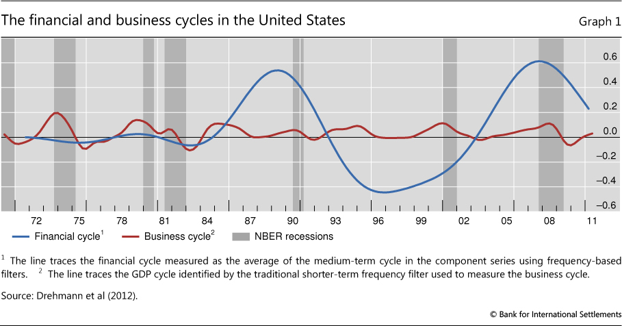
Importantly, the relevant cycle for the instrument is not the business cycle but the "financial cycle" - the boom and bust cycles that characterise the financial system. Aikman et al (2010), Claessens et al (2011) and Drehmann et al (2012) document that financial variables (in particular, credit and property prices) have pronounced and largely coincident cycles. These financial cycles have greater amplitude and duration than the fluctuations in economic activity, known as the business cycle. Graph 1 (taken from Drehmann et al (2012)) illustrates this for the United States. More often than not, financial cycle peaks are punctuated by banking crises. The CCB aims to help banks survive such episodes. However, the CCB is not a tool intended to actively manage the cycle. The Basel Committee notes the instrument's "potential moderating effect on the build-up phase of the credit cycle" but characterises this as no more than "a positive side benefit" (BCBS (2010, page 1)).
Repullo and Saurina (2011) argue that the credit gap is not the right anchor for the buffer because it moves countercyclically with GDP growth. Their argument places the business cycle centre stage and suggests that a CCB driven by the credit gap would exacerbate rather than smooth fluctuations in GDP. There are both statistical and economic counterarguments against this criticism.
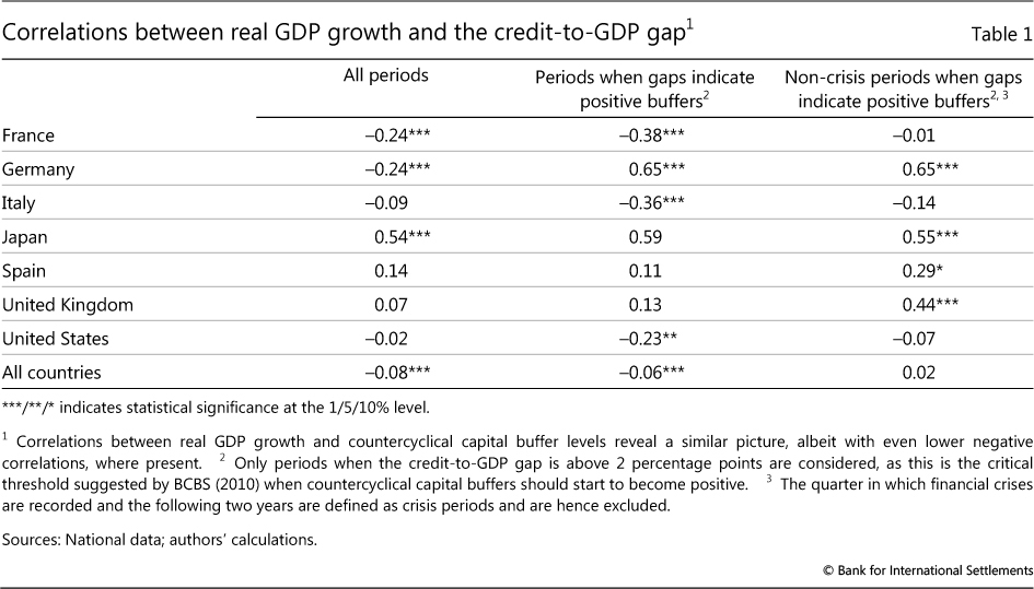
From a statistical point of view, the criticism regarding the correlation between the credit gap and real GDP growth is only partly correct. This correlation is indeed negative across a panel of 53 countries over the period 1980-2013 but small in size (Table 1, first column).3 Closer examination of the data reveals that the negative sign is driven primarily by periods when the information from the indicator is of no consequence for the capital buffer. These are either periods during which the credit gap was low and the capital buffer would not have been activated, or periods following crises when the buffer would have been released. Excluding these periods renders the correlation either positive or statistically indistinguishable from zero (Table 1, second and third columns).
More importantly, the starting point of the criticism is incorrect. The value of a guide for the CCB must be assessed against the buffer's economic objectives, which is not to manage the business cycle, but to defend banks against the financial cycle.
To be sure, the lack of coincidence between financial and business cycles does raise challenges. There have been periods when the credit gap would have suggested increasing capital buffers in the midst of a recession. And a decision to increase the countercyclical buffer in such times, even if justified on prudential grounds, may meet with stiff political resistance. But, even in these circumstances, it is unclear how strong the real impact on GDP would be: the empirical literature fails to provide evidence of a strong link between higher bank capital requirements and lower growth. Recent studies put the median estimates for the impact of a 1 percentage point increase in capital requirements on GDP in the range of 0.1 to 0.2 percentage points, while the long-term impact of better capitalised banks on economic output is estimated to be positive (BCBS (2010)).4
Edge and Meisenzahl (2011) as well as Buncic and Melecky (2013) point out that the credit-to-GDP gap is not necessarily an equilibrium notion of credit for the economy. These authors agree with the idea that the CCB should protect banks from the consequences of financial booms, but they express doubt that the credit gap can correctly identify periods of "excessive" credit growth.
This is a valid point in the sense that no formal model underpins the choice of this indicator, but it does not imply that the measure entirely lacks theoretical foundations or that is not fit for purpose. Conceptually, the credit gap encapsulates the build-up of financial vulnerabilities in line with the ideas of Kindleberger (2000) and Minsky (1982) about the mechanisms that lead to crises. Empirically, it is consistent with a growing literature documenting that unusually strong credit growth tends to precede crises (Schularick and Taylor (2012), Gourinchas and Obstfeld (2012)). Furthermore, given that the function of the credit gap is not to set a target for aggregate credit but to guide the build-up of bank capital ahead of problems, it should be judged solely on its indicator properties for incipient banking stress. We discuss those in the next section.
Is the credit-to-GDP gap the best EWI for banking crises?
Many authors have proposed indicators other than the credit gap as anchors for the CCB (eg Barrell et al (2010), Shin (2013), Behn et al (2013)). They argue that their preferred alternative to the credit-to-GDP gap works better as an EWI for banking crises. In this section, we review the evidence in favour of the credit-to-GDP gap.
Predicting banking crises is an exercise in compromise. The ideal indicator would signal all impending crises and never crises that fail to materialise. All known EWIs fall short of this ideal, and hence they must be evaluated on the basis of how they trade off the rate of missed crises against the rate of false positives (ie the percentage of signals they emit for crises that do not happen). This evaluation depends on policymakers' preferences concerning these two types of error.
Good EWIs must fulfil a number of additional requirements that go beyond statistical accuracy. Drehmann and Juselius (2014) propose three such requirements in the context of macroprudential policymaking. The first is timing: EWIs must provide signals early enough for policy measures to take effect. For instance, the Basel III guidance states that "the indicator should breach the minimum [critical threshold] at least 2-3 years prior to a crisis" (BCBS (2010, page 16)). The second requirement is stability: the indicator should not flip-flop between signalling a crisis and being "off". EWIs that issue stable signals reduce uncertainty regarding trends and allow for more decisive policy actions. The final requirement is interpretability. Forecasts and signals that policymakers find hard to understand and interpret are likely to be ignored (eg Önkal et al (2002), Lawrence et al (2006)). This puts a premium on simplicity and ease of communication, making single indicators with robust performance particularly appealing.
The credit gap fares well against these criteria. As we discuss below, it is the EWI of banking crises, having the best overall statistical performance among single indicators across a large panel of countries over the past several decades. It also satisfies the three policy requirements listed above, and its calculation requires data (credit and GDP) which are generally available in most jurisdictions. These characteristics are essential considering that the BCBS guidance underpins a globally harmonised framework.
We use a panel of 26 countries over the period 1980-2012 to compare the performance of six indicators: the credit-to-GDP gap, credit growth, GDP growth, residential property price growth, the debt service ratio (DSR) and the non-core liability ratio.5 The DSR is defined as the proportion of interest and amortisation payments to income and was first suggested in this context by Drehmann and Juselius (2012). The non-core liability ratio was proposed by Hahm et al (2012) and captures the reliance of a banking system on wholesale and cross-border funding.6
We follow Drehmann and Juselius (2014) in evaluating the forecast performance of EWIs using the area under the curve (AUC): a statistical methodology that captures the trade-off between true positives and false positives for the full range of policymakers' preferences (see box for a description). A completely uninformative indicator has an AUC of 0.5: it is no better than tossing a coin. The greater the difference of the AUC from 0.5, the better the forecast performance of the indicator. For indicators whose value increases ahead of crises, the perfect AUC score would be equal to 1. For indicators that decline ahead of crises, the perfect AUC score would be zero. Importantly for the problem at hand, the AUC is robust to a technical issue that complicates regression-based assessments. Variables that satisfy the stability requirement, which is desirable from a policy perspective, are bound to be very persistent (ie move very smoothly over time). This persistence complicates the statistical evaluation of their forecasting power on the basis of standard regression models, such as those used by Barrell et al (2010).7
Evaluating EWIs with the AUC
The AUC (the area under the receiver operating characteristics curve, or ROC curve) is a statistical tool used in assessing the performance of signals that forecast binary events (ie events that either occur or do not). The term ROC reflects the origins of the tool in the analysis of radar signals during World War II, although it has a long tradition in other sciences (eg Swets and Picket (1982)). Its applications to economics are more recent (eg Cohen et al (2009), Berge and Jorda (2011), Jorda et al (2011)). The AUC summarises the trade-off between correct and false signals for all different operator (policymaker) preferences, as explained below.
Selecting an indicator involves making a choice on the trade-off it offers between the rate of correct event predictions and the rate of false calls. There are four possible value combinations of a binary signal (which can be "on" or "off") and subsequent event realisations ("occurrence" or "non-occurrence"). The perfect indicator signals "on" ahead and only ahead of all occurrences, while the signal from an uninformative indicator has an equal probability of being right or wrong. Signals from continuous variables (such as those considered in this article) must be calibrated. This means that the operator will define a threshold and consider as a signal a value of the indicator variable that exceeds this threshold. Varying the threshold varies the relationship between true positives (signal "on" and "event occurs") and false positives (signal "on" and "non-occurrence"). If it is set at a very high value, the indicator will miss many events but it will also make very few false positive signals. A very low threshold value will generate many signals, capturing more events but also making many more false calls.
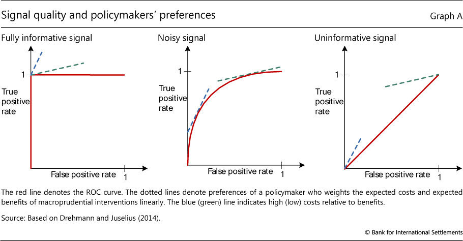
The ROC curve for an indicator captures the relationship between the rate of true positives (as a share of all occurrences) and the rate of false positives (as a share of all non-occurrences) for different values of the threshold. The red lines in the graph below illustrate the ROC curve for three different indicators. The left-hand panel corresponds to the perfect indicator. Since the indicator is able to perfectly signal occurrences, decreasing the threshold value from the maximum implies that more and more events are predicted without any false calls being made (vertical segment). When the threshold is set so as to capture all occurrences, lowering it further will not increase the rate of correct predictions, which is already at 1, but will add to the rate of false calls (horizontal segment). The right-hand panel shows the other extreme: the completely uninformative indicator. Lowering the threshold in this case changes the true positive and false positive rates, but always by the same amount. The trade-off is thus depicted by the 45° line. The more interesting cases are between the extremes (centre panel): as calibration moves away from the origin of the graph (by lowering the threshold from its maximum value), it initially improves the true positive rate at a low cost in terms of increases in the false positive rate. The cost of improving the true positive rate, however, increases (the ROC curve flattens) as the threshold is progressively lowered.
The operator (the policymaker) is not indifferent about this trade-off and assigns a positive weight to the success rate (correct predictions of occurrences) and a negative weight to the rate of false positives. These preferences are shown as straight lines. The steeper (blue dotted) line corresponds to an operator who dislikes false positives relatively more than another operator who is more interested in not missing an occurrence (green dotted line). Each operator tries to achieve the highest extension of the slope that represents their preferences. For the two extreme cases, the choice is trivial. In the case of the fully informative indicator, all operators will select the calibration that offers perfect accuracy. In the case of the uninformative indicator, the two operators will position themselves at opposite ends: one at the point of zero false positives and zero success rate (the origin), and the other at the point where all occurrences are captured but also the false positive rate is 100%. In realistic situations of informative but noisy indicators, each operator will select a different calibration as seen by the points of tangency in the centre panel. For each operator, the distance between the red line at the point of tangency and the 45° line represents the gain they obtain given their preferences and the options offered by the specific indicator.
The AUC is calculated as the area under the entire ROC curve. Intuitively, it captures the average gain over the uninformed case across all possible preferences of the operator (ie for all possible combinations of weights assigned to the two types of error). As such, it provides a summary measure of the signalling quality over the full range of possible preferences and calibrations (Elliott and Lieli (2013)). This is particularly appealing given the difficulties of offering precise quantification of the costs and benefits of macroprudential policymaking (CGFS (2012)). The uninformative indicator has an AUC equal to 0.5 (area under the 45° line), while that for the fully informative indicator is equal to 1. The intermediate cases have values in between. For indicators that decline ahead of events, the AUC takes values between 0.5 (uninformative) and zero (fully informative).
This assumes that the indicator increases ahead of an event. If the opposite is true, then a signal is "on" when the variable is below the threshold and the explanation is reversed.
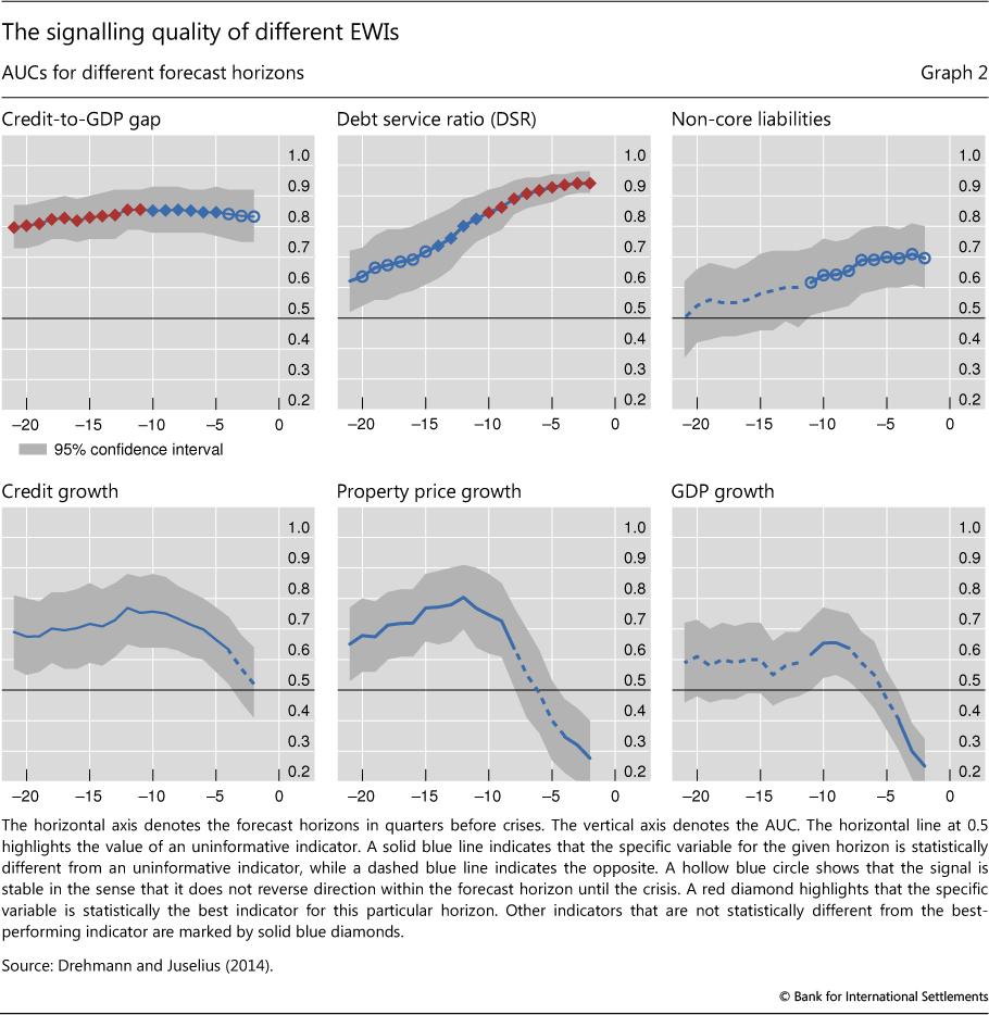
Graph 2 shows the AUC metric for the six EWIs over forecast horizons that range from 20 quarters to one quarter prior to a banking crisis. A solid blue line indicates that the specific variable for the given horizon is statistically different from an uninformative indicator, while a dashed blue line indicates that a variable is statistically indistinguishable from an uninformative indicator. We use circles and diamonds to indicate the ranking of performance among the six indicators for a given forecast horizon. For each horizon, the best-performing indicator (ie the one with the highest AUC) is denoted by a red diamond. A blue diamond denotes that the specific variable is not statistically different from the best-performing indicator. A blue circle shows that the signal is stable in the sense that it does not reverse direction within the forecast horizon until the crisis.
The clear message from Graph 2 is that, among those considered, the credit-to-GDP gap is statistically the best single EWI for forecast horizons between five and two years. At shorter horizons, the best single indicator is the DSR. The other indicators have an inferior performance to these two and often fail to satisfy the stability property.
The credit-to-GDP gap as a mechanical anchor for the CCB
Given its overall robust performance, should the CCB be anchored mechanically on the credit-to-GDP gap? The answer is no, for a number of reasons. For one, since no indicator is infallible, policymaking requires judgment. For another, combinations of indicators perform better than single ones. And, as many observers have pointed out, what works best for the entire panel might work for most countries and periods but not necessarily for all individual situations.
As with other countercyclical policies, including monetary policy, decisions incorporate a substantial element of judgment. A rules-based, mechanical approach has attractions, especially when it comes to dealing with political economy problems, but it also has pitfalls, because all indicators and models are subject to error and the future is, by definition, unknown. The uncertainties in the context of CCB decisions are no different. The role of the credit gap in the CCB framework is not that of a rigid benchmark, but that of a guide: an easy-to-calculate indicator that can facilitate the communication between the policymaker, the banks and the public. It should work as a yardstick to anchor judgment and explain the rationale for decisions. It is not meant to be the one-size-fits-all benchmark for CCB application, but a source of discipline in the application of judgment by national authorities.
Combinations of indicators could also act as benchmarks. Indeed, research points to composite indicators that statistically outperform the credit-to-GDP gap. For instance, Borio and Lowe (2002) as well as Behn et al (2013) found that combinations of the credit gap and a similarly calculated asset price gap produce a more precise signal, while Drehmann and Juselius (2014) found complementary information content in the debt service ratio. Yet problems with universal data availability for such indicators and additional framework complexity argued in favour of adopting a simpler, single indicator as guide for the CCB.
A number of jurisdictions that have implemented the framework have made the case for using indicators that better capture the specific circumstances of their financial system. For instance, the Bank of England (2014) has introduced a framework that is based on 18 core indicators, including the credit gap. Similarly, the Swiss National Bank (2013), the Central Bank of Norway (2013) and the Reserve Bank of India (2013) have explained that they monitor a small number of indicators in addition to the credit gap in evaluating aggregate vulnerabilities and making decisions regarding the CCB.8 As in the Bank of England's approach, these additional indicators relate primarily to conditions in the residential and commercial property markets and sometimes include bank liabilities.
Others have argued that the credit gap is not appropriate in a particular country at a given point in time (eg Reserve Bank of South Africa (2011), Wolken (2013)). The latter type of argument must be carefully backed by analysis, as there is a temptation to generalise from episodes when the gap gave wrong signals. This in and of itself does not invalidate the early warning properties of the credit gap, as these can be assessed only in a larger sample. And its superior cross-country performance sets a high bar for such arguments, suggesting that they would be the exception rather than the rule. The background analysis must also tackle the challenge of a small sample: statistical assessments for single countries are difficult given the low number of crises (generally two or fewer).
Noise in the signal produced by the credit gap in specific circumstances may occur in periods when the ratio increases because of a collapse in the denominator (GDP) rather than a surge in the numerator (credit). This tends to occur in the early stages of a recession. As discussed above, the mechanical use of the indicator could produce unintended effects in these situations, but this risk is low given the room for discretion provided by the framework and the fact that the CCB would not be active in most of those situations. Nevertheless, Kauko (2012) suggests using a five-year moving average instead of current GDP levels in the denominator of the ratio as a way of minimising the problem of sudden falls in GDP. This approach could reduce the number of wrong signals in recessions, but results in a credit gap with a somewhat lower AUC compared with those using actual GDP. So, reducing the rate of false positives when a fall in GDP is the driver of the increase comes at the cost of lower overall predictive ability.9
Ironically, the adoption of the credit gap as an anchor for policy decisions may eventually weaken its signalling properties without invalidating its function as a guide. Goodhart (1975) postulated that a variable used to guide policy may lose its information content precisely because it is embedded in the policy framework. In an ideal world where signals are accurate and policy responses perfectly gauged, the building of capital buffers would protect banks against the build-up of vulnerabilities but may also defuse the underlying risks, and thus weaken the statistical link between the credit gap and crises. But this should be seen as a sign of success and not negate the usefulness of the indicator for policy, or be interpreted as a reason to abandon the CCB altogether.10
Is the credit-to-GDP gap a good early warning indicator for emerging market economies?
A number of commentators question the usefulness of the credit-to-GDP gap as a guide in the case of emerging market and transition economies (eg Geršl and Seidler (2012)). They point out that the evidence provided by BCBS (2010) and previous research (eg Drehmann et al (2011)) is based on samples comprising largely advanced economies. Sceptics also argue that emerging market economies (EMEs) are more likely to be undergoing a period of financial deepening which renders the specification of the trend for the calculation of the credit gap problematic (eg World Bank (2010)). We deal with these issues in turn.
We present evidence that the performance of the credit gap as an EWI carries over to a sample of EMEs, albeit this performance is not as good as it is for the sample that includes advanced economies. To this end, we constructed an enlarged panel of 53 countries with data starting at the earliest in 1980. In doing so, we had to overcome two issues.
The first relates to data availability, a common challenge in implementing the CCB in EMEs. For many EMEs, credit statistics are either not available for longer time spans (we need at least 20 years of data in order to properly assess the forecasting ability of the credit gap), or they are plagued by structural breaks. As we show in the next section, these breaks can affect very strongly the credit gap calculation. For 32 countries, we use total credit to the private non-financial sector from the BIS database.11 For another 21 countries, we use bank credit to the private non-financial sector from the IMF's International Financial Statistics, requiring that data are available quarterly (as this suggests a minimum of data quality) and for at least three years prior to a crisis.
The second issue has to do with the classification of economies as advanced or emerging markets. For robustness, we split the sample in two different ways. The first simply classifies countries into emerging market and advanced economies. The second is based on the level of the credit-to-GDP ratio: we classify countries with a ratio below the (arbitrary) threshold of 100% as EMEs.12 Both classifications have their shortcomings, but the thrust of the results is not sensitive to the choice.13
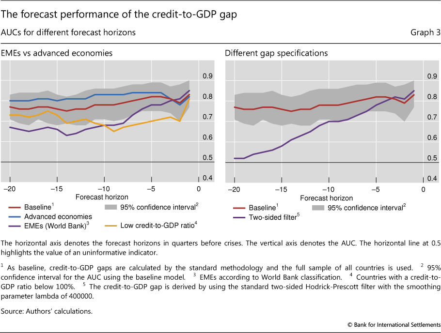
The left-hand panel of Graph 3 shows the performance of the credit-to-GDP gap as an early warning indicator for the two groups of countries. It plots the AUC for the indicator estimated for different country samples and different forecasting horizons.
The credit gap performs well for EMEs, albeit not as well as it does for the group of advanced economies. Regardless of the classification approach for EMEs (purple and yellow lines), the AUC remains above the 0.5 threshold, although it is below the level that corresponds to the sample of advanced economies (blue line). In fact, for forecasting horizons greater than three years, the AUC is marginally better than the uninformative benchmark value of 0.5. This deterioration in performance is very likely driven by the small number of crises in the EME samples (no more than 10 episodes in either classification).
Another criticism of the credit gap with respect to its applicability for EMEs is that it may hinder beneficial financial deepening. As pointed out in World Bank (2010) or Reserve Bank of India (2013), economies that go through the process of financial development can experience prolonged periods of credit growth. To the extent that credit growth exceeds past norms, it could trigger increases in the CCB that could be a drag on further deepening and slow the process of catching up with financially more advanced economies.
This issue relates to the calculation of the long-run trend. If financial deepening occurs at a steady pace, a gradual and persistent growth of credit will be embedded in the trend of the credit-to-GDP ratio and will not affect the gap. By contrast, rapid expansions of credit are likely to be flagged by the credit-to-GDP gap as periods of financial vulnerabilities. The flip side of this is that a protracted credit boom will weaken the credit gap's signalling ability, an aspect that concerns also advanced economies (Wolken (2013)). A prolonged but large steady increase in the credit-to-GDP ratio will eventually lead to a lower credit gap without necessarily implying that financial stability risks have receded. For example, the credit gap in the Netherlands signalled vulnerabilities from 1998 to 2004, but a systemic banking crisis emerged only in 2008 (admittedly also due to cross-border factors).
These problems highlight the risk from a mechanical use of the credit gap. Policymakers have to assess whether in these situations credit levels are sustainable or whether they are a source of aggregate vulnerability. In practice, and in line with the Basel III proposal, this can only be done by looking at a range of different indicators rather than relying on any mechanical rule.
Measurement problems and the credit-to-GDP gap
Several authors have argued that the performance of the credit-to-GDP gap can be severely hampered by measurement problems. The majority of these problems relate to the calculation of the long-term trend of the ratio. We will tackle them first, before briefly commenting on measurement noise from statistical revisions relating to the ratio itself.
Basel III specifies that the long-term trend of the credit-to-GDP ratio should be calculated using the time series filter suggested by Hodrick and Prescott (1981) (HP filter) with a suitably large smoothing parameter. Critics have pointed to two potential measurement problems in this calculation. The first problem is linked to the stability of the filter's outcome as new data points become available. The second problem arises because structural breaks in the underlying series can have an important effect on the calculation of the trend. We discuss these aspects below.
Following the original work by Borio and Lowe (2002), the long-term trend of the credit-to-GDP ratio is calculated by means of a one-sided (ie backward-looking) HP filter. The filter is run recursively for each period, and the ex post evaluation of performance of the credit gap is based on this recursive calculation. Thus, a trend calculated for, say, end-1988 only takes account of information up to 1988 even if this calculation is done in 2008 when more observations have become available. As specified in Basel III, the filter uses a much larger smoothing parameter than the one employed in the business cycle literature involving quarterly data.14 This choice can be motivated by the observation that credit cycles are on average about four times longer than standard business cycles and crises tend to occur once every 20-25 years.15 It turns out that this specific choice of the smoothing parameter also delivers the credit-to-GDP gap with the best forecasting performance (Drehmann et al (2011)).
The HP filter suffers from a well-known end point problem.16 This means that the estimated trend at the end point (the most recent observation) can change considerably as future data points become available. Since Basel III prescribes that the trend be calculated recursively, policy decisions are always based on a trend that consists only of end points. Edge and Meisenzahl (2011) argue that the backward revision of the trend (and, by consequence, also the deviation of the ratio from the trend) renders the credit gap unreliable as a guide for the CCB.
Drehmann et al (2011) and van Norden (2011) note that the end point problem does not invalidate the signalling ability of the credit-to-GDP gap. From a practical perspective, it would be impossible for the policymaker to apply a two-sided filter since the future is not observable. But even if policymakers did somehow know the future values of the credit-to-GDP ratio and calculated credit gaps based on this knowledge, the resulting indicator would not outperform the gap calculated with the backward-looking HP filter except for exceedingly short forecast horizons of less than four quarters (purple line in Graph 3, right-hand panel). For policy-relevant horizons, the gap based on the one-sided filter (red line) performs much better than the gap calculated with the two-sided filter. Nevertheless, Gerdrup et al (2013) suggest an alternative approach to the problem of trend stability. At each end point, they extend the sample by five years with forecasts of the credit-to-GDP ratio and calculate a two-sided filter for this augmented series. They find that the resulting credit gap has good forecasting performance for Norway. By contrast, Farrell (2013) finds that this approach worsens the credit gap's performance, especially during pronounced credit booms.
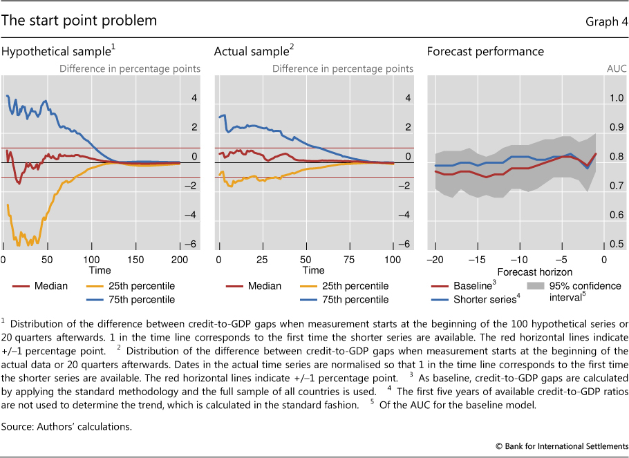
A similar problem arises at the beginning of the time series used to compute the credit gap. Geršl and Seidler (2012) point out that the trend calculation can depend significantly on the starting point of the data. This is particularly important for short data series, which is the case in several EME countries. To assess the severity of this problem more formally, we use an estimated time series model to generate 100 artificial series of credit-to-GDP ratios, each 400 quarters long.17 For each of these hypothetical series, we computed two series for the credit-to-GDP gap: one starting from the beginning of the simulated data, and another starting 20 quarters later. We then compare the two gap series for the 380 observations over which the two overlap. In line with this approach, we also estimate a second series of gaps for our actual data, starting 20 quarters after the first observation of the credit-to-GDP ratio in each country.
Graph 4 shows that the starting point for estimating the trend can have major implications for the measurement of the gap. While the median difference between the two gaps across the 100 hypothetical series is less than half a percentage point after 40 quarters, the 25th and 75th percentiles of the distribution of simulated differences show gaps of up to 4 percentage points at the same horizon (left-hand panel). The problem is less severe when we use actual data from our panel (centre panel), although even in this case it can take 20 years for measurement differences to fully disappear.
But in practice, the impact of this mismeasurement is not as great as the above figures suggest. For one, the forecast performance of the two differently derived gaps in the actual data is the same (Graph 4, right-hand panel). Furthermore, even if there are differences in the gaps, the differences in the resulting CCB levels are small. If one were to apply the Basel III rule mechanically, the CCB is set to zero for values of the credit gap below 2 percentage points and capped at 2.5% for values of the gap above 10. Given this transformation, the difference in the CCB levels driven by the start point problem is 0 in most cases after 10 years. Even at extreme ends of the distribution, the difference is smaller than 1 percentage point.
Overall, these results validate the practical rule of thumb that suggests using the credit gap only when at least 10 years of data for the credit-to-GDP ratio are already available. This was originally suggested by Borio and Lowe (2002) and adopted in BCBS (2010).
In particular situations, caution is warranted nonetheless. Closer examination of the simulated data shows that large differences between the gaps calculated on shorter and longer samples tend to arise in situations where the shorter sample starts near the peak or the trough of the financial cycle. In these instances, the trend stays too high or too low for a long period. This was the case for transition economies during the 1990s. In these contexts, policymakers may consider dropping some initial data points. As more data become available, the problem becomes less important for policymaking, although it remains an issue for the ex post assessment of the performance of the credit gap.
Structural breaks in the credit-to-GDP series present similar challenges to the start point problem discussed above (FitchRatings (2010), World Bank (2010)). Graph 5 (left-hand panel) illustrates the effect of such a statistical break assuming that the credit-to-GDP ratio jumps by 10 percentage points. The Japanese total credit series registered a break of similar magnitude in 1998 due to a change in the way the series was compiled. The simulation shows that it takes more than 20 years for such an effect of this magnitude to fully disappear, underscoring the importance of properly adjusting the underlying series for breaks prior to use as a guide for policy.18
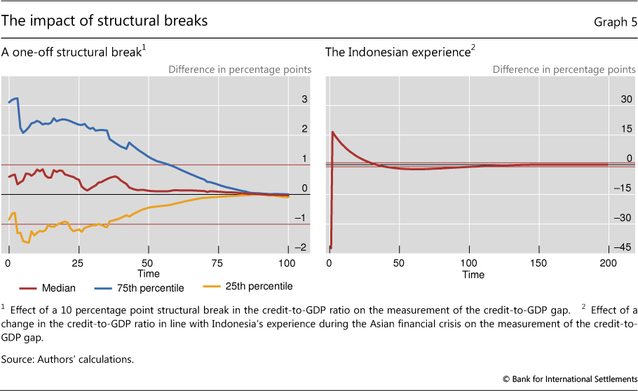
Economic factors can also create jumps in the credit-to-GDP series similar to statistical revisions. For example, during the Asian crisis, in Indonesia a combination of foreign currency loans, rapid devaluation and large-scale defaults led to a 50 percentage point jump in the credit-to-GDP ratio followed by a 6 percentage point drop. A simulation of this very dramatic swing (Graph 5, right-hand panel) suggests that such events can impact the measurement of the credit-to-GDP gap for around 10 years. Their influence on the signalling function of the credit gap must be understood prior to the series being used in the context of the CCB.
Lastly, another measurement issue is linked to routine statistical revisions in the underlying data. This is a problem with economic variables that policymakers often have to grapple with. In the case of the credit gap, the main concern is that it can impair its signalling performance. Edge and Meisenzahl (2011) carefully evaluate the impact of revisions to the credit-to-GDP gap in the United States and find that they have an impact on gap estimates. However, they also find that this impact is contained and much smaller than variations in the trend estimate due to the end point problem, discussed above. Gerdrup et al (2013) and Farrell (2013) argue along the same lines for Norwegian and South African data, respectively.
Conclusion
We have reviewed the main practical and conceptual criticisms of the credit-to-GDP gap as a guide to setting countercyclical capital buffers under Basel III.
From a practical perspective, there are relevant measurement issues with the credit gap, which critics have pointed out. In particular, the length of the underlying series for the credit-to-GDP ratio and thus the starting point for calculating the trend matter. Structural breaks in the credit-to-GDP ratio can also have long-lasting effects. Our simulations indicate that it is important to properly adjust the data for structural breaks. In addition, a valid rule of thumb suggests using the credit gap only for credit-to-GDP series with at least 10 years of available data.
We argue that the conceptual criticism that the credit gap is not aligned with the buffer's objective misinterprets this objective and, by extension, the envisaged role of the guide. The CCB framework provides supervisors with an instrument to increase capital in order to protect banks from the bust phase of the financial cycle. It is not an instrument to manage the cycle, even if it may potentially have a smoothing impact. From this viewpoint, its usefulness must be judged exclusively on whether it provides policymakers with reliable signals about when to raise the buffer. Reviewing the evidence, we show that the credit-to-GDP gap is on average (across many countries and several decades) the best single indicator in this context, including for emerging market economies. This does not mean that there are no composite indicators that may perform better, or single indicators that may provide clearer signals either in the context of individual countries or at particular points in time. But it does mean that even in those cases the credit gap is a very useful common reference point and helps frame the discussion.
This is a central feature of a CCB framework which combines rules and discretion. There are no foolproof models that can deliver an effective rule-based countercyclical instrument. Policymakers are expected to use judgment as well as quantitative analysis within the parameters of the framework. But they are also expected to communicate the rationale of their decisions clearly. The credit gap can be instrumental in this process.
References
Aikman, D, A Haldane and B Nelson (2010): "Curbing the credit cycle", paper prepared for the Columbia University Centre on Capital and Society Annual Conference, New York, November.
Bank of England (2014): The Financial Policy Committee's powers to supplement capital requirements - a Policy Statement, January.
Barrell, R, E Davis, D Karim and I Liadze (2010): "Calibrating macroprudential policy", NIESER Discussion Papers, no 354.
Basel Committee on Banking Supervision (2010): Guidance for national authorities operating the countercyclical capital buffer, December.
Behn, M, C Detken, T Peltonen and W Schudel (2013): "Setting countercyclical capital buffers based on early warning models: would it work?", ECB Working Paper Series, no 1604, November.
Berge, T and O Jorda (2011): "Evaluating the classification of economic activity into recessions and expansions", American Economic Journal: Macroeconomics, vol 3(2), pp 246-77.
Borio, C and M Drehmann (2009): "Assessing the risk of banking crises - revisited", BIS Quarterly Review, March, pp 29-46.
Borio, C and P Lowe (2002): "Assessing the risk of banking crises", BIS Quarterly Review, December, pp 43-54.
______ (2004): "Securing sustainable price stability: should credit come back from the wilderness?", BIS Working Papers, no 157.
Buncic, D and M Melecky (2013): "Equilibrium credit: the reference point for macroprudential supervision", World Bank, Policy Research Working Paper, no 6358, February.
Central Bank of Norway (2013): "Criteria for an appropriate countercyclical capital buffer", Norges Bank Papers, no 1/2013.
Claessens, S, M Kose and M Terrones (2011): "How do business and financial cycles interact?", IMF Working Papers, no WP/11/88.
Cohen, J, S Garman and W Gorr (2009): "Empirical calibration of time series monitoring methods using receiver operating characteristic curves", International Journal of Forecasting, no 25(3), pp 484-97.
Committee on the Global Financial System (2012): "Operationalising the selection and application of macroprudential instruments", CGFS Publications, no 48.
Drehmann, M (2013): "Total credit as an early warning indicator for systemic banking crises", BIS Quarterly Review, June, pp 41-5.
Drehmann, M, C Borio and K Tsatsaronis (2011): "Anchoring countercyclical capital buffers: the role of credit aggregates", BIS Working Papers, no 355.
______ (2012): "Characterising the financial cycle: don't lose sight of the medium term!", BIS Working Papers, no 380.
Drehmann, M and M Juselius (2012): "Do debt service costs affect macroeconomic and financial stability?", BIS Quarterly Review, September, pp 21-34.
______ (2014): "Evaluating early warning indicators of banking crises: satisfying policy requirements", International Journal of Forecasting, forthcoming (also BIS Working Papers, no 421).
Edge, R and R Meisenzahl (2011): "The unreliability of credit-to-GDP ratio gaps in real-time: implications for countercyclical capital buffers", International Journal of Central Banking, December, pp 261-98.
Elliott, G and R Lieli (2010): "Predicting binary outcomes", Journal of Econometrics, no 174, pp 15-26.
Farrell, G (2013): "Countercyclical capital buffers and real-time credit-to-GDP gap estimates: a South African perspective", mimeo.
FitchRatings (2010): Macro-Prudential Risk Monitor, June.
Gerdrup, K, A Kvinlog and E Schaanning (2013): "Key indicators for a countercyclical capital buffer in Norway - trends and uncertainty", Central Bank of Norway (Norges Bank), Staff Memo, no 13/2013, Financial Stability.
Geršl, A and J Seidler (2012): "Excessive credit growth and countercyclical capital buffers in Basel III: an empirical evidence from central and east European countries", Economic Studies and Analyses, no 6(2).
Goodhart, C (1975): "Monetary relationships: a view from Threadneedle Street", Reserve Bank of Australia, Papers in Monetary Economics, vol I.
Gourinchas, P-O and M Obstfeld (2012): "Stories of the twentieth century for the twenty-first", American Economic Journal: Macroeconomics, no 4(1), pp 226-65.
Hahm, J-H, H S Shin and K Shin (2012): "Non-core bank liabilities and financial vulnerability", mimeo.
Hodrick, R and E Prescott (1981): Post-war US business cycles: an empirical investigation.
Jorda, O, M Schularick and A Taylor (2011): "When credit bites back: leverage, business cycles and crises", Federal Reserve Bank of San Francisco, Working Papers, no 2011-27.
Kauko, K (2012): "Triggers for countercyclical capital buffers", Bank of Finland Online, no 7.
Kindleberger, C (2000): Maniacs, panics and crashes, Cambridge University Press, Cambridge.
Lawrence, M, P Goodwin, M O'Connor and D Önkal (2006): "Judgmental forecasting: a review of progress over the last 25 years", International Journal of Forecasting, no 22(3), pp 493-518.
Minsky, H (1982): Can "it" happen again? Essays on instability and finance, M E Sharpe, Armonk.
Önkal, D, M Thomson and A Pollock (2002): "Judgmental forecasting", in M Clements and D Hendry (eds), A companion to economic forecasting, Blackwell Publishers, Malden and Oxford.
Orphanides, A and S van Norden (2002): "The unreliability of output-gap estimates in real time", Review of Economics and Statistics, no 84(4), pp 569-83.
Park, J and C Phillips (2000): "Nonstationary binary choice", Econometrica, vol 68(5), pp 1249-80.
Ravn, M and H Uhlig (2002): "On adjusting the Hodrick-Prescott filter for the frequency of observations", Review of Economics and Statistics, vol 84(2), pp 371-6.
Repullo, R and J Saurina (2011): The countercyclical capital buffer of Basel III: a critical assessment.
Reserve Bank of India (2013): "Report of the internal working group on implementation of countercyclical capital buffer", draft, December.
Reserve Bank of South Africa (2011): Financial Stability Report, September. Schularick, M and A Taylor (2012): "Credit booms gone bust: monetary policy, leverage cycles and financial crises, 1870-2008", American Economic Review, vol 102(2), pp 1029-61.
Shin, H S (2013): "Procyclicality and the search for early warning indicators ", IMF Working Papers, no 13/258.
Swets, J and R Picket (1982): Evaluation of diagnostic systems: methods from signal detection theory, Academic Press, New York.
Swiss National Bank (2013): Implementing the countercyclical capital buffer in Switzerland: concretising the Swiss National Bank's role.
Van Norden, S (2011): "Discussion of 'The unreliability of credit-to-GDP ratio gaps in real-time: implications for countercyclical capital buffers'", International Journal of Central Banking, December, pp 300-3.
Wolken, T (2013): "Measuring systemic risk: the role of macro-prudential indicators", Reserve Bank of New Zealand Bulletin, vol 76, no 4.
World Bank (2010): Comments on the consultative document countercyclical capital buffer proposal.
1 We thank Claudio Borio, Juan Carlos Crisanto, Dietrich Domanski, Tamara Gomes and Christian Upper for very helpful comments, as well as Angelika Donaubauer and Michela Scatigna for excellent research assistance. The views expressed are those of the authors and do not necessarily reflect those of the BIS.
2 See eg Borio and Drehmann (2009), FitchRatings (2010), Behn et al (2013) and Drehmann and Juselius (2014).
3 See the next section for a more detailed description of the data used in this article.
4 For a recent overview, see CGFS (2012).
5 Using somewhat different techniques, Drehmann et al (2011) found that indicators of banking sector performance (eg aggregate non-performing loans) and market-based indicators (eg credit spreads) perform poorly. Drehmann and Juselius (2014) also consider real equity price growth and gaps of property and equity prices that are not shown here for the sake of brevity.
6 In line with the findings of Hahm et al (2012), the non-core liability ratio is empirically measured by cross-border liabilities plus M3 minus M2 (proxy for non-core liabilities) divided by M2 (proxy for core liabilities).
7 Park and Phillips (2000) offer a discussion of how series persistence can lead to misleading inference in binary choice models.
8 All three institutions use these indicators expressed in "gap" form, that is, in terms of the difference between their current value and their respective long-term trend.
9 We have performed analysis that demonstrates this for our panel of countries. The results are available upon request.
10 See Drehmann et al (2011).
11 Basel III suggests the use of data on total credit, capturing not only bank credit but all sources of credit, including bonds and cross-border finance, to the private non-financial sector. Drehmann (2013) shows that the credit gaps based on total credit outperform the credit gaps based on bank credit as early warning indicators for banking crises. Total credit series are available at http://www.bis.org/statistics/credtopriv.htm.
12 If the credit-to-GDP ratio breaches 100% in the run-up to a crisis, this episode is considered to be part of the low credit-to-GDP sample.
13 EME = emerging market economy. Adv = advanced economy. <100 = credit-to-GDP ratio below 100%. If given, the date indicates the quarter when the ratio breached 100%. Algeria (EME, <100), Australia (Adv, <100 1986q2), Austria (Adv, <100 1990q2), Belgium (Adv, <100 1990q3), Brazil (EME, <100), Bulgaria (EME, <100), Canada (Adv, <100 1980q1), Chile (EME, <100), China (EME, <100 1998q2), Colombia (EME, <100), Croatia (EME, <100), the Czech Republic (EME, <100), Denmark (Adv, <100 1980q1), Estonia (EME, <100 2009q2), Finland (Adv, <100 1985q4), France (Adv, <100 1990q2), Germany (Adv, <100 1981q1), Greece (Adv, <100 2007q2), Hong Kong SAR (EME, <100 1988q4), Hungary (EME, <100 2005q4), Iceland (Adv, <100 2002q1), India (EME, <100), Indonesia (EME, <100 1998q1), Ireland (Adv, <100 1993q1), Israel (Adv, <100), Italy (Adv, <100 2005q3), Japan (Adv, <100 1980q1), Korea (EME, <100 1984q4), Latvia (EME, <100), Lithuania (EME, <100), Malaysia (EME, <100 1990q4), Mexico (EME, <100), the Netherlands (Adv, <100 1980q3), New Zealand (Adv, <100 1997q4), Norway (Adv, <100 1980q1), Peru (EME, <100), the Philippines (EME, <100), Poland (EME, <100), Portugal (Adv, <100 1980q1), Romania (EME, <100), Russia (EME, <100), Saudi Arabia (EME, <100), Singapore (EME, <100 1985q4), South Africa (EME, <100), Spain (Adv, <100 1981q3), Sweden (Adv, <100 1980q1), Switzerland (Adv, <100 1985q2), Thailand (EME, <100 1991q1), Turkey (EME, <100), the United Arab Emirates (EME, <100), the United Kingdom (Adv, <100 1987q3), the United States (Adv, <100 1982q3) and Venezuela (EME, <100).
14 Hodrick and Prescott (1981) set λ equal to 1600. Ravn and Uhlig (2002) show that, for series of other frequencies (daily, annual etc), it is optimal to set λ equal to 1600 multiplied by the fourth power of the observation frequency ratio. Borio and Lowe (2002) suggest that, for the credit-to-GDP gap, λ be set equal to 400000.
15 See BCBS (2010).
16 See eg Orphanides and van Norden (2002).
17 The model postulates that the credit-to-GDP ratio follows an AR(2) process with positive drift. Its coefficients and error variance are estimated using a random-effects regression for our panel of countries.
18 The new BIS total and bank credit series are available as raw and break-adjusted series.