Under pressure: market conditions and stress

When financial markets come under pressure, vital functions such as the efficient allocation of capital and price formation become impaired¹. It is therefore important to enhance the monitoring and analysis of market conditions, in particular events that may put pressure on authorities to intervene. We introduce market conditions indicators (MCIs) for each of three key market segments: the US Treasury and US money markets, and the foreign exchange market centred around the US dollar. Our daily MCIs reflect market volatility, illiquidity and deviations from standard no-arbitrage conditions. They capture well known episodes of market turmoil. We show that it is in some cases possible to identify conditions that point to a heightened risk of future market stress months ahead of the event.

JEL classification: G10, G17, G21, G23.

Since the Great Financial Crisis (GFC), structural changes in financial markets have significantly altered the nature of liquidity provision. For one, banks have adapted to a new regulatory environment that limits their ability to warehouse risks. At the same time, the heft of non-bank financial institutions (NBFIs) has risen markedly (Carstens (2021), Aramonte et al (2021)). In addition, technological improvements have facilitated high-speed trading on automated platforms (Markets Committee (2022)).

In this environment, episodes of market stress have become more frequent and widespread. We treat "stress" as a broad concept, covering periods of market dysfunction as well as periods when markets are functioning but amid liquidity that is low in historical terms.²  Stress episodes are characterised by impairments to price formation and the breakdown of no-arbitrage relationships. From a policy perspective, it is important to monitor any deterioration of market conditions in real time and, in combination with leading indicators, to anticipate a potential need for intervention before stress has begun.

This special feature develops separate daily market conditions indicators (MCIs) for three key markets: the US Treasury market, US money markets and the foreign exchange (FX) market centred around the US dollar. These markets are key for monetary policy implementation and the fulfilment of central bank mandates. Furthermore, they are distinct yet intertwined, not least in the modern market-based financial system where money market funding of capital market lending supported by collateral plays a key role (Mehrling et al (2013)). We focus on the United States – and by extension the dollar – due to its central role in global financial markets.

We construct each MCI in two steps and use it to define stress episodes, focusing on one market at a time. First, we identify variables that capture market illiquidity or deviations from standard no-arbitrage conditions. Second, we equate an MCI with the factor that explains most of the variation across these variables. We define market stress as realisations of the MCI that fall in the upper tail of its historical distribution. The three MCIs spike concurrently when stress is pervasive, but also identify market-specific stress episodes. They co-move only loosely with the VIX, with which alternative indicators of financial conditions or stress are tightly linked.

Next, we examine the extent to which it is possible to anticipate MCI realisations that indicate stress. We are interested in uncovering leading indicators that signal market fragility and are associated with an elevated risk of future market stress, rather than in predicting the exact timing of stress episodes.³  We consider two broad categories of variables that may signal fragilities: one capturing investors' overextension and risk perceptions, the other reflecting more structural features of markets such as intermediaries' market-making capacity and funding liquidity conditions. Our results suggest that it is possible in some cases to identify (in sample) a heightened probability of stress several months prior to the event.

The rest of this article is organised as follows. The first section briefly discusses conceptual issues around the measurement of market conditions and stress, contrasting our approach with the related literature. The second presents the construction of our three MCIs and discusses their properties. A third section assesses the probability of future stress. The final section concludes with policy considerations.

Financial conditions, vulnerabilities and stress

The GFC gave new impetus to the study of financial market conditions and stress, and their effect on the economy at large.⁴  But as the adage goes, "not everything that can be counted counts, and not everything that counts can be counted". Market conditions certainly count, but are hard to "count": they are critical, yet not directly observable.

In practice, measurement difficulties have translated into a variety of financial stress (FSIs) and conditions indices (FCIs).⁵ These have similarities, but also important differences in terms of both inputs and scope (Monin (2017)). Both FSIs and FCIs combine information from various financial variables into a single number. FSIs focus on identifying distress and dysfunction as they occur. They are often constructed with financial market prices only. By contrast, FCIs were originally designed to measure the impact of financial conditions on the economy and therefore tend to have a medium-term focus (Hatzius et al (2010), Adrian et al (2022)). Furthermore, FCIs tend to incorporate information on quantities in addition to financial market prices.

Our approach to measuring market conditions is close to the one underpinning FSIs. An important goal of our approach is to identify episodes of market stress as they occur, with stress broadly understood as poor market conditions. As such, we aim for coincident rather than early warning indicators. In addition, we use daily series with near real-time availability and hence focus almost exclusively on financial market prices as inputs.

That said, our approach also differs from that behind most FSIs in a number of dimensions, most notably regarding input variables. For one, we focus on disruptions to market liquidity, mispricing and the breakdown of standard arbitrage relations that are the tell-tale sign of impaired market functioning. Unlike FSIs, we do not consider variables from the equity market (eg valuations and volatility). Furthermore, our approach is more parsimonious than that of alternative indices. At a practical level, this simplifies collection and maintenance. At a conceptual level, it brings the virtue of greater transparency and greater scope for understanding the general state of market conditions. Finally, we also differ in our focus on individual key markets that are interwoven by the role of market-making and collateral to support leveraged strategies. Our approach thus aligns with the type of interventions central banks have made in recent times as dealers of last resort to backstop specific asset markets.

Measuring market conditions

We construct the MCIs in two steps. First, for each of the three markets, we collect variables capturing volatility, market (il-)liquidity and funding (il-)liquidity as well as impaired market-making more broadly. We aim to strike a balance between the coverage of different aspects of market conditions and availability of a reasonably lengthy daily time series. Guided by this trade-off, we start our analysis in 2003.

The specific variables we consider are well known (online annex Table A). Those that capture market dislocation reflect the breakdown of no-arbitrage conditions. Examples include the cross-currency basis in FX markets,⁶ or deviations of observed bond yields from a fitted smooth yield curve in the Treasury market. Measures of market liquidity, in turn, aim to capture the ease with which market participants can trade without significantly affecting prices. Examples include quoted bid-ask spreads for spot FX or the premium between on- and off-the-run Treasury securities. Finally, we incorporate measures of market uncertainty, such as the JPMorgan FX volatility indices and the MOVE index for the FX and Treasury markets, respectively.

The variables capture, to different degrees, known episodes of poor market conditions over the past two decades. For example, FX market volatility and dislocation measures, such as the JPMorgan FX volatility index or deviations from covered interest parity (CIP)⁷ (Du et al (2018), Rime et al (2022)), signalled the European sovereign debt crisis in 2011–12, the 2015 de-pegging of the Swiss franc from the euro, Brexit and the US money market fund (MMF) reform (Graph 1, left-hand panel). In the Treasury market, measures of market liquidity (eg the time it takes dealers to provide quotes) and volatility (eg the MOVE index) rose around the GFC, taper tantrum, Covid-19 pandemic and the start of the war in Ukraine (centre panel). Similar measures also play a role in money markets. The spreads between repo and overnight index swap (OIS) rates (market dislocation) and between high-quality financial commercial paper and OIS rates (market liquidity) surged during the GFC, the US MMF reform, the VIX spike in early 2018, the September 2019 repo turmoil and the pandemic (right-hand panel).

In the second step, we build market-specific composite indicators. We express all variables so that higher values indicate worse market conditions and use principal component analysis (PCA) to extract a common factor from them.⁸  The MCI for each market is defined as the first principal component, ie the linear combination of the underlying series that captures most of their variability. For ease of interpretation, we normalise the MCIs to have zero mean and unit standard deviation. Accordingly, positive values reflect tighter than average market conditions.

Our MCIs capture both broad-based and market-specific episodes.⁹  All three MCIs spiked (though to differing degrees) during the GFC and the Covid-19 crisis (Graph 2). But they also indicated material deterioration of market conditions outside these most severe episodes. For example, the FX MCI picked up during the European sovereign debt crisis in 2011–12 and from 2015 to 2016 following the Swiss franc de-peg, Brexit and the US MMF reform. The Treasury MCI, in turn, inched up slightly into positive territory following the taper tantrum in 2013 as well as during the flash events of 2014 and 2021.¹⁰  It has been rising quickly since early 2022 (see below). Finally, the money market MCI remained largely subdued outside the GFC and the Covid-19 crisis. That said, it did exhibit moderate increases around some episodes, such as the MMF reform and the 2018 VIX spike.

Comparing the three indicators can shed light on how conditions differed across markets at any given point in time (Graph 3).¹¹  Ahead of the Lehman collapse, for example, it was Treasury, and especially money market, turmoil that led the way, with FX market conditions sharply deteriorating only afterwards. In contrast, tighter than average FX market conditions dominated during the European sovereign debt crisis, Brexit and around the US MMF reform. More recently, tight market conditions were most visible in the Treasury market, with values approaching the levels seen during the GFC (though still well below the Covid-19 turmoil). This development is in line with recent commentary on declining Treasury market liquidity (Federal Reserve Board (2022), Scheicher and Schrimpf (2022)).

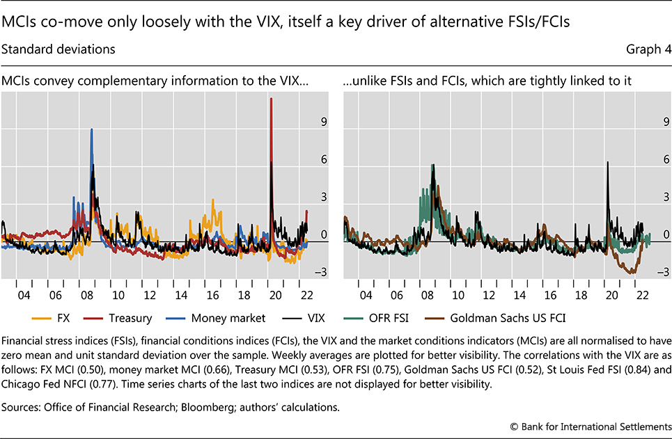
Importantly, our MCIs do not simply capture information already reflected by the VIX – as is the case for most FCIs/FSIs. While the MCIs are positively linked with the VIX, there are instances in which they convey distinct information (Graph 4, left-hand panel). One example is the already discussed rise in the FX MCI during 2015–16, a period that did not exhibit a commensurate increase in the VIX. Conversely, the VIX remained elevated in the aftermath of the Covid-19 turmoil, whereas all three MCIs pointed to a swift reversal to benign market conditions. More broadly, the focus of the MCIs allows them to highlight different intensities in the deterioration of market conditions across markets and time.¹²  In contrast, FSIs and FCIs are in general very tightly linked to the VIX (right-hand panel).¹³  This is not surprising, since the VIX is an input in their construction. But as the VIX is only one among dozens of input variables, its tight link with FSIs and FCIs is striking.

All in all, our market-specific MCIs are related to, but distinct from, commonly used FSIs, FCIs and the VIX.

Measuring the probability of future stress

Given the importance of well functioning financial markets for the real economy, policymakers have an interest in understanding how stress risk builds up, and ideally in anticipating stress episodes. This is especially so since the severity of recent stress events has prompted authorities to backstop markets (Markets Committee (2022)).

However, any attempt to forecast episodes of market stress will face non-trivial challenges, especially over horizons long enough to allow for pre-emptive policy action. These range from difficulties in identifying leading indicators to structural changes in markets that may affect such indicators' information content. Moreover, as is clear from our MCIs, there are several large spikes that correspond to inherently unpredictable events, such as Covid-19, the outbreak of war in Ukraine and various flash events (Graph 2). Predicting the exact timing of such shocks is simply impossible.

It may therefore be more fruitful to attempt to uncover conditions that signal an increased likelihood of future market stress by indicating market fragility. Information that broadly captures investor overextension (excessive search for yield, big changes in investor flows, atypically low levels of volatility etc) should be useful in revealing fertile ground for future stress. Using such information would be in the spirit of the literature on early warning indicators of banking crises (Borio and Drehmann (2009), Aldasoro et al (2018)).¹⁴  Signals of investors' perceptions of elevated market risk would also be useful, as they speak directly to what we are interested in: the likelihood of a stress event. Such variables are typically tightly linked to, or may simply be mirror images of, those capturing overextension: a sudden withdrawal of investors in the face of unsustainable conditions would be a clear signal of heightened risk. We thus group all these variables into one category.

A second group of variables we consider is of a more structural nature. Here, we aim to capture information that need not be related to investor overextension or risk perceptions, but that still may have a bearing on future market stress. This includes information on the market-making capacity of intermediaries, as well as indicators measuring funding liquidity conditions in markets.

The time horizon matters for the information content of leading indicators. Specific signs of overextension would typically take time to surface as stress – or, alternatively, dissipate. At the same time, the explanatory power of any variable tends to vanish at long horizons. In turn, indicators of investor risk perceptions tend to be useful over shorter horizons. Information on liquidity conditions and market-making capacity may be informative over both short and long horizons, depending on how persistent the underlying drivers are. With this in mind, we focus on horizons between one month and one year when assessing future stress risk.¹⁵

Methodology

We use a logit model to examine the extent to which one can identify developments that signal a heightened risk of future market stress. In our setting, this amounts to modelling the odds of future "stress" relative to "no stress" as a function of a set of explanatory variables. Once we have estimated the parameters of the logit model, we calculate implied stress probabilities for each of the three markets we consider and compare them with actual stress episodes.

Our empirical model requires that we first construct a discrete variable that signals stress or no stress in the market. We do this by simply defining stress periods as the months when a given MCI is in the top 20% of its values over the sample period.¹⁶  The choice of a 20% cutoff involves a trade-off. It is sufficiently high to avoid a focus only on a few severe events, but still low enough to capture all periods with a meaningful degree of stress.

When selecting indicators that can help explain a rising risk of future stress, we focus on variables in the two categories discussed above: (i) those that point to investor overextension or that signal perceptions of higher risk in the market; and (ii) variables which are informative about liquidity conditions and market-making capacity.¹⁷  Most variables are common to all three market segments, as they signal broad financial developments. Others have narrower informational content and are thus included only for some markets (online annex Table B).

Overextension / risk perception

Starting with variables that broadly capture investors' overextension and risk perceptions, we consider both quantity and price-based data. On the quantity side, we use information on exchange-traded fund (ETF) and investment fund flows. Strong flows to certain sectors or asset classes can point to shifts in investors' risk appetite. Insofar as the shifts are unsustainable, they may be helpful in signalling risks of sudden reversals and market stress further down the road. Conversely, sudden large outflows can point to perceptions of heightened market uncertainty.

We consider intra-family investor flow shifts from one type of mutual fund to another. An example is shifts towards high-yield bond mutual funds as suggested by Ben-Rephael et al (2021; BCG henceforth). BCG argue that such flow shifts are due to changes in investors' risk appetite. For our purposes, this may be useful information if increased risk-taking raises the likelihood of a future reversal and associated market stress. We also include a related measure by Ben-Rephael et al (2012; BKW henceforth), capturing investors' sentiment through shifts between bond and equity funds.¹⁸ Finally, we consider total ETF inflows, which may capture similar information.

We include two price-based measures of investor overextension. One is the global financial cycle (GFCy) of Miranda-Agrippino and Rey (2020), which summarises fluctuations across hundreds of global asset prices and strongly interacts with monetary and financial conditions, including booms and busts.¹⁹  The second measure is the US broad dollar index (DXY), which has been found to be tightly linked to funding and liquidity conditions as well as to the risk-taking behaviour of global banks (see, among others, Shin (2016) and Avdjiev et al (2019a,b)).

In turn, we consider two variables that may capture market participants' perceptions of higher market risk. The first one is the VIX, which incorporates investors' expectations of near-term equity market volatility. An elevated VIX could point to possible market fragilities due to perceptions of higher risk. The second variable in this category is margin requirements, which tend to increase with market uncertainty and may therefore be useful in signalling stress. Specifically, we use CME initial margins on 10-year Treasury futures.²⁰  Importantly, the same indicators but at different values may signal the build-up of imbalances: prolonged periods when the VIX is low or margins are overly compressed may stem from increased risk-taking and leveraging-up.

Liquidity conditions / market-making capacity

Next, we consider variables reflecting liquidity conditions and intermediaries' market-making capacity. One such variable is the excess bond premium (EBP) of Gilchrist and Zakrajšek (2012) – a corporate credit spread shown to be informative about the risk-bearing capacity of the financial sector. A deterioration in risk-bearing capacity (signalled by a rise in the EBP) is likely to result in greater market fragility and a higher likelihood of future stress. We also include the net holdings of Treasury bonds by primary dealers. Du et al (2022) argue that in the post-GFC environment, when dealers maintained systematically net long Treasury positions, this variable served as a reliable indicator of dealers' balance sheet constraints. More constrained dealers have less room to arbitrage mispricings, potentially leaving markets more vulnerable to future stress. Having said that, a reduction in primary dealer Treasury holdings could also reflect a withdrawal from the market as a result of perceived greater uncertainty, which in turn could foreshadow stress in the Treasury market itself.²¹

We consider two additional variables that could affect liquidity conditions across market segments. The Federal Reserve's purchases of Treasuries may be important for conditions in both the Treasury and money markets. In particular, it is a key determinant for whether liquidity is ample or not. The total issuance of commercial paper (CP) can also affect conditions in funding markets by altering the portfolio composition of money market investors. A rise in CP issuance would, all else equal, reduce investments in other market segments, potentially reducing their liquidity.

Besides the above two categories of variables, we also include lagged values of the MCIs for the three markets we consider. By doing so, we hope to account for any persistence as well as possible spillovers and co-dependencies across market segments.

In the logit analysis, we successively narrow down the set of explanatory variables for each market segment by excluding those that are (mostly) statistically insignificant. The only variable that drops out from all three markets is, perhaps surprisingly, the VIX.²²  All other variables remain for at least one market segment.

Logit results: implied stress probabilities

Graph 5 displays the stress probabilities implied by the logit model estimates for each of the three market segments. These refer to the probability of stress occurring six months ahead.^{23, 24}  The graph shows that the model can identify (in sample) a higher stress probability ahead of a number of stress episodes.²⁵

Consider, for example, the run-up to the GFC-related stress in money markets. Our classification scheme dates the start of this stress episode as August 2007 (Graph 5, left-hand panel), when BNP Paribas froze three of its ABS investment funds and the dollar interbank market began seizing up. The model-implied stress probability rose quickly in the run-up to this episode: while the six-month-ahead stress probability stood at below 5% around mid-2006, it had risen to 50% six months before the episode started, and all the way to 75% by June 2007. Our estimates show that the main driver of this increase was a strong rise in the global financial cycle variable GFCy.^{26, 27}  A rising BGC indicator, measuring investor flow shifts towards high-yield bond mutual funds, contributed as well, even if to a lesser extent.²⁸  Both of these variables indicated increasingly aggressive risk-taking, which in turn signalled a rising risk of sudden reversal and attendant market stress.

A second example comes from the FX market, which saw stress concentrated in late 2015 and through much of 2016, preceded by a gradual rise in the estimated stress probability (Graph 5, centre panel). During this time, markets were unsettled as the Federal Reserve was preparing for its eventual December interest rate lift-off, while global growth prospects were deteriorating. In the FX MCI, this manifested itself through eg rising bid-ask spreads and widening CIP deviations.²⁹  Our classification method identifies November 2015 as the start of the stress episode. While the six-month-ahead stress probability had hovered around 5–10% at end-2014, it rose to 37% six months prior to the start of the stress episode, and to above 60% in the last months leading up to it. An increasing EBP credit spread was important in explaining the rise of the model-implied probability, suggesting that reduced financial sector risk-bearing capacity played an important role. Moreover, greater risk-taking and possible investor overextension seemed to also contribute to the build-up in the stress probability, as indicated by a general rise in BKW investment flow shifts and total ETF inflows prior to the episode.³⁰  Finally, a rise in lagged FX MCI values played an increasingly important role in the lead-up to the stress episode. This suggests that the build-up of stressed FX market conditions was gradual.

A more recent example is the Treasury market stress of 2022, which kicked off in March according to our classification. A key reason for the onset of stress was the start of the war in Ukraine in late February. In the face of already high inflation rates, the resulting commodity price spike contributed to an acceleration in planned quantitative tightening and other contractionary moves by the Fed.³¹  While the exact timing of the stress event was unpredictable, the fact that our estimated stress probability began to rise months ahead points to pre-existing fragility (Graph 5, right-hand panel). The estimated six-month-ahead stress probability went from essentially zero at the start of 2021 to 47% six months prior to the stress episode and 64% three months before. Taken at face value, these results suggest that the market stress was in the making, and the war outbreak was the trigger that pinned down the timing.

Looking under the hood, we see that market participants' expectations of looming stress played an important role in the recent increase in Treasury market stress probability. The DXY dollar index contributed due to ongoing dollar strengthening at the time. This was largely linked to rising US bond yields that mean widespread bond market losses, greater market uncertainty and rising fragility. Linked to this, primary dealers were reducing their net holdings of Treasuries, possibly in anticipation of market stress.^{32, 33}  Moreover, initial margins on Treasury futures were rising, consistent with growing market uncertainty. In this increasingly fragile environment, CP issuance was also rising, thereby directing capital away from other segments, including the Treasury market.

Conclusion

The rising frequency and reach of market stress episodes call for enhancing authorities' ability to monitor market conditions and analyse stress risk in financial markets. We propose a new set of market conditions indicators for three key market segments and use them to define stress episodes.

From a policy perspective, it is key to have a warning when the risk of future stress increases. We examine whether variables capturing investor overextension and perceptions of risk, as well as indicators of funding liquidity conditions and market-making capacity, could be helpful in this regard. All in all, our results show that by exploiting the information captured by such variables, it is in some cases possible to anticipate increased market stress risk.

These results, however, should be interpreted with caution. Importantly, our findings are based on an in-sample exercise. Out-of-sample evaluations are beyond our scope, but represent an important topic for future research because they underpin real-time forecasts for policymaking. Further analyses could also delve more deeply into the information content of rising implied probabilities, not least by contrasting correct anticipation of stress with false alarms and missed stress episodes. More broadly, any set of results from a focused exercise, such as the one in this article, should be but one component in a holistic understanding of market developments.

References

Adrian, T, F Grinberg, N Liang, M Sheheryar and J Yu (2022): "The term structure of growth-at-risk", American Economic Journal: Macroeconomics, vol 14, pp 283–323.

Aldasoro, I, C Borio, M Drehmann (2018): "Early warning indicators of banking crises: expanding the family", BIS Quarterly Review, March, pp 29–45.

Aramonte, S, A Schrimpf and H S Shin (2021): "Non-bank financial intermediaries and financial stability", BIS Working Papers, no 972, October.

Aronovich, A, D Dobrev and A Meldrum (2021): "The Treasury market flash event of February 25, 2021", FEDS Notes.

Avdjiev, S, V Bruno, C Koch and H S Shin (2019a): "The dollar exchange rate as a global risk factor: evidence from investment", IMF Economic Review, vol 67, no 1,pp 151–73.

Avdjiev, S, W Du, C Koch and H S Shin (2019b): "The dollar, bank leverage, and deviations from covered interest parity", American Economic Review: Insights, vol 1, no 2, pp 193–208.

Ben-Rephael, A, J Choi and I Goldstein (2021): "Mutual fund flows and fluctuations in credit and business cycles", Journal of Financial Economics, vol 139, pp 84–108.

Ben-Rephael, A, S Kandel and A Wohl (2012): "Measuring investor sentiment with mutual fund flows", Journal of Financial Economics, vol 104, pp 363–82.

Bisias, D, M Flood, A Lo and S Valavanis (2012): "A survey of systemic risk analytics", Annual Review of Financial Economics, vol 4, pp 255–96.

Board of Governors of the Federal Reserve System (Federal Reserve Board) (2022): Financial Stability Report, May.

Borio, C and M Drehmann (2009): "Assessing the risk of banking crises - revisited", BIS Quarterly Review, March, pp 29–46.

Borio, C, M Iqbal, R McCauley, P McGuire and V Sushko (2016): "The failure of covered interest parity: FX hedging demand and costly balance sheets", BIS Working Papers, no 590 (revised November 2018).

Carlson, M, K Lewis and W Nelson (2014): "Using policy intervention to identify financial stress", International Journal of Finance & Economics, vol 19, pp 59–72.

Carstens, A (2021): "Non-bank financial sector: systemic regulation needed", BIS Quarterly Review, December, pp 1–6.

Christensen, J, J Lopez and P Shultz (2017): "Do all new Treasuries trade at a premium?", FRBSF Economic Letter, 2017-03.

Davis, J and A Zlate (2022): "The global financial cycle and capital flows during the COVID-19 pandemic", Federal Reserve Bank of Dallas Globalization Institute Working Paper, no 416.

Du, W, B Hébert and L Wen (2022): "Intermediary balance sheets and the Treasury yield curve", NBER Working Paper, no 30222.

Du, W, A Tepper and A Verdelhan (2018): "Deviations from covered interest parity", The Journal of Finance, vol 73, no 3, pp 915–57.

Gilchrist, S and E Zakrajšek (2012): "Credit spreads and business cycle fluctuations", American Economic Review, vol 102, pp 1692–720.

Greenwood, R, S Hanson, A Shleifer and J Sørensen (2022): "Predictable financial crises", The Journal of Finance, vol 77, pp 863–921.

Hatzius, J, P Hooper, F Mishkin, K Schoenholtz and M Watson (2010): "Financial conditions indexes: A fresh look after the financial crisis", NBER Working Paper, no 16150.

Huang, W, A Ranaldo, A Schrimpf and F Somogyi (2021): "Constrained dealers and market efficiency", University of St Gallen School of Finance Research Papers, 2021/16.

Kliesen, K, M Owyang and E Vermann (2012): "Disentangling diverse measures: a survey of financial stress", Federal Reserve Bank of St Louis Review, vol 94, no 5, pp 369–97.

Markets Committee (2022): Market dysfunction and central bank tools, May.

Mehrling, P, Z Pozsar, J Sweeney and D Neilson (2013): Bagehot was a shadow banker: shadow banking, central banking, and the future of global finance.

Miranda-Agrippino, S and H Rey (2020): "US monetary policy and the global financial cycle", The Review of Economic Studies, vol 87, no 6, pp 2754–76.

Monin, P (2017): "The OFR Financial Stress Index", Office of Financial Research Working Papers, no 17-04.

Rime, D, A Schrimpf and O Syrstad (2022): "Covered interest parity arbitrage", The Review of Financial Studies, forthcoming.

Scheicher, M and A Schrimpf (2022): "Liquidity in bond markets – navigating in troubled waters", SUERF Policy Brief, no 395, August.

Shin, H S (2016): "The bank/capital market nexus goes global", speech at the London School of Economics and Political Science, 15 November.

Tarashev, N, K Tsatsaronis and C Borio (2016): "Risk attribution using the Shapley value: methodology and policy applications", Review of Finance, vol 20, no 3, pp 1189–213.

---

Online annex

---

¹ The authors thank Claudio Borio, Stijn Claessens, Mathias Drehmann, Benoît Mojon, Andreas Schrimpf, Hyun Song Shin, Fabricius Somogyi, Vladyslav Sushko, Nikola Tarashev and Philip Wooldridge for valuable comments and suggestions, Pietro Patelli for excellent research assistance, and Azi Ben-Rephael and co-authors as well as Douglas Richardson from the Investment Company Institute for kindly sharing data. The views expressed in this article are those of the authors and do not necessarily reflect those of the Bank for International Settlements.

² For a definition of market dysfunction, see Markets Committee (2022).

³ This is in line with common practice in financial stability analysis: focus on assessing vulnerabilities, not triggers of stress episodes.

⁴ Two related areas of work that saw a post-GFC resurgence are that of early warning indicators of banking crises (Borio and Drehmann (2009), Greenwood et al (2022)) and systemic risk measurement (Bisias et al (2012), Tarashev et al (2016)).

⁵ See Hatzius et al (2010), Carlson et al (2014) and Kliesen et al (2012) for literature reviews.

⁶ The cross-currency basis denotes the difference between the interest paid to borrow one currency by swapping it against another and the cost of directly borrowing this currency in the cash market. A non-zero value indicates a violation of covered interest parity.

⁷ These series also help illustrate the importance of the institutional environment. CIP deviations were non-existent before the GFC. Rising hedging demand and tighter limits to arbitrage post-GFC turned CIP deviations into a structural feature of financial markets (Borio et al (2016)).

⁸ Before performing the PCA analysis, we put all variables on an equal footing through a z-score transformation (ie subtracting the sample mean and dividing by the sample standard deviation).

⁹ The first principal component that equals the FX MCI accounts for around 43% of the variance of the input series; the corresponding shares are 46% and 65% for the Treasury and money market MCIs.

¹⁰ Aronovich et al (2021) review the 2021 flash event and compare it with previous episodes.

¹¹ The MCIs are not additive. Hence, Graph 3 combines them for illustrative purposes only.

¹² Examples include a sharper rise in the money market and Treasury MCIs at the start of the GFC and a considerably larger increase in the Treasury MCI during Covid-19.

¹³ For brevity, we focus on the most well known financial conditions and stress indicators, namely the FSI from the Office of Financial Research (OFR) and the FCI from Goldman Sachs. Alternative FSIs and FCIs deliver a very similar, and sometimes crisper, message. Goldman Sachs' FCI is strongly influenced by equity prices, which explains its divergence from the VIX and OFR FSI during the substantial equity rally that followed the Covid-19 market turmoil.

¹⁴ We discuss a number of such variables in some detail in the following subsection.

¹⁵ Such horizons are much shorter than those studied in the literature on financial crises, which is concerned with the slow build-up of fragility in the system that can accumulate over years. Market stress and the conditions leading to it, in contrast, are arguably of a shorter nature.

¹⁶ We aggregate the daily MCIs into monthly (non-overlapping) averages in order to avoid a focus on short-lived spikes. The use of a monthly frequency also allows us to extend the set of potential explanatory variables beyond high-frequency market prices.

¹⁷ Table B in the online annex provides a summary of all explanatory variables considered.

¹⁸ Inspired by Ben-Rephael et al (2012, 2021), we also use Investment Company Institute data to construct a measure of intra-family flow shifts into MMFs to capture potential investor overextension in money markets (referred to as "MM flow shifts" in online annex Tables B and C).

¹⁹ The GFCy variable is only publicly available up to 2018. We therefore rely on the approximation suggested by Davis and Zlate (2022) and compute the first principal component of weekly equity returns for a sample of 48 countries (22 advanced and 26 emerging market economies). When aggregated at the monthly frequency, this measure has a correlation of 0.9 with Miranda-Agrippino and Rey's GFCy indicator.

²⁰ This variable is thus specific to the Treasury market; unavailability of data precluded inclusion of margin information for the other market segments.

²¹ This indicator could therefore potentially straddle both variable categories.

²² The VIX is only significant at the very shortest horizons, ie one to two months, as a sudden rise in the VIX is often associated with already occurring market stress, which in turn has some near-term persistence. Over longer horizons, of greater policy relevance, it plays no significant role.

²³ We calculate implied stress probabilities up to 12 months ahead, but here focus on the six-month horizon for brevity. These results are broadly representative of those at other horizons. Online annex Tables C–E display our logit parameter estimates for the three-, six-, nine- and 12-month horizons.

²⁴ The last observation for the probabilities in Graph 5 is December 2021 (six months prior to the end of our sample), ie the last month for which we can evaluate the probabilities against an outcome.

²⁵ Across the 12 horizons we consider, the McFadden pseudo-R² values range from 44 to 63% for the money market, from 62 to 80% for the Treasury market, and from 25 to 69% for the FX market.

²⁶ The parameter estimates corresponding to this variable are positive across all horizons (and significant for three-month and longer horizons), in line with it conveying information about investor risk-taking, possible overextension and heightened risk of a reversal (see online annex Table C).

²⁷ Throughout, we judge the importance of the drivers based on the extent to which they raise the stress probability during the relevant episode (keeping everything else unchanged).

²⁸ While the coefficient for BCG is not statistically significant for the six-month horizon, it is significant (and consistently positive) for longer horizons (see online annex Table C).

²⁹ The 2015 year-end was the first one after leverage ratio disclosure rules came into effect, which may have played a role. Bank balance sheet contractions at reporting periods (quarter-ends and especially year-ends) became frequent thereafter, with ripple effects across FX markets. In addition, the early implementation of the US MMF reform started in April 2016, adding pressure to FX and money markets through the final implementation date in October 2016.

³⁰ In line with our interpretation, the parameter estimates for EBP, BKW flow shifts and ETF inflows are all positive across every horizon (online annex Table D).

³¹ This was also occurring against the backdrop of ongoing structural changes in liquidity provision in the Treasury market. Since 2020, the composition of the domestic investor base has changed: commercial banks have increased their presence while long-term investors such as insurers have pulled back (see the Overview).

³² These two factors can also interact with each other. This occurs if the selling of Treasuries by central bank reserve managers – eg to lean against the wind of a strengthening dollar – increases the volume that comes to the market precisely when intermediation capacity is low.

³³ Interestingly, the logit parameter estimates for primary dealer holdings are negative (when significant) for the Treasury market, in line with our interpretation of the role this variable played for the probability of Treasury stress (online annex Table E). Instead, for the other two markets the parameter estimates are positive, consistent with the original mechanism described in the "Methodology" section above (online annex Tables C and D).