The financial cycle and recession risk
Financial cycle booms can end in crises and, even if they do not, they tend to weaken growth. Given their slow build-up, do they convey information about recession risk? We compare the predictive performance of different financial cycle proxies with that of the term spread - a popular recession indicator. In contrast to much of the literature, our analysis covers a large sample of advanced and emerging market economies. We find that, in general, financial cycle measures provide valuable information and tend to outperform the term spread.1
JEL classification: C33, E37, E44.
Once financial cycles peak, the real economy typically suffers. This is most evident around financial crises, which tend to follow exuberant credit and asset price growth, ie financial cycle booms. Crises in turn tend to usher in deep recessions, as falling asset prices, high debt burdens and balance sheet repair drag down growth.
This suggests that the financial cycle could be helpful for gauging recession risk, in particular as booms are drawn out and exhibit systematic patterns. Given the tight link between crises and recessions, this seems to be implied by the large body of work on the leading indicator properties of financial booms for banking crises (eg Borio and Drehmann (2009), Schularick and Taylor (2012) and Detken et al (2014)). Some studies have also documented that credit booms weaken output in the medium run (eg Mian et al (2017) and Lombardi et al (2017)). And some recent work has begun to study the impact of financial conditions on risks to growth (eg Adrian et al (2018)).2
But research exploring how financial expansions affect recession risk, ie the likelihood that a recession will develop in the near future - say, one to three years ahead - is scant and predominantly focused on the United States.3 Assessing recession risk has a long tradition. Probably the most popular variable in this context is the term spread (eg Estrella and Mishkin (1998) and Rudebusch and Williams (2009)). In particular, an inverted yield curve - long-term bond yields below short-term interest rates - is seen as among the best signals of impeding recessions, if not the best.
Key takeaways
- We evaluate how far financial cycle proxies can assess recession risks in a large sample of advanced and emerging market economies.
- We find that the proxies provide valuable information even at a three-year horizon.
- Financial cycle proxies generally outperform the term spread.
In this special feature, we examine the ability of financial cycle proxies to convey information about recession risk. We follow the literature very closely to better benchmark our analysis against the corresponding work on the term spread. In contrast to much of the extant analysis, we look at a large sample of advanced and emerging market economies (EMEs).4
For advanced economies, we find that financial cycle proxies provide valuable information for a horizon of up to three years, outperforming the term spread. The evidence for EMEs mirrors that for advanced economies, although data limitations prevent out-of-sample tests for this group.
The rest of the article is structured as follows. In the first section, we briefly introduce the notion of the financial cycle and document how the nature of the business cycle, and its link with the financial cycle, have changed in the past 50 years. In the second, we explain our methodology. In the third, we evaluate the performance of financial cycle proxies and compare it with that of the term spread based on full-sample information, ie ex post. In the fourth, we consider out-of-sample exercises, seeking to mimic the information policymakers have when assessing risks in real time, ie ex ante.
A look at the data
The term "financial cycle" refers to the self-reinforcing interactions between perceptions of value and risk, risk-taking, and financing constraints (Borio (2014)). Typically, rapid increases in credit drive up property and asset prices, which in turn increase collateral values and thus the amount of credit the private sector can obtain until, at some point, the process goes into reverse. This mutually reinforcing interaction between financing constraints and perceptions of value and risks has historically tended to cause serious macroeconomic dislocations.
The financial cycle can be approximated in different ways. Empirical research suggests that, especially if one is interested in episodes that have proven more damaging for economic activity, a promising strategy is to capture it through medium-term fluctuations in credit and property prices. This can be done either in terms of individual series or, preferably, of their combination. In this special feature, we rely on a "composite" financial cycle proxy similar to that in Drehmann et al (2012). In addition, as an alternative, we also look at the debt service ratio, defined as interest payments plus amortisation divided by GDP.5 Drehmann et al (2018) find a strong link between debt accumulation and subsequent debt service (ie interest payments plus amortisation), which in turn has a large negative effect on growth.6
Previous research has identified two important features of the financial cycle.7 First, financial cycle peaks tend to coincide with banking crises or considerable financial stress. This is not surprising. During expansions, the self-reinforcing interaction between financing constraints, asset prices and risk-taking can overstretch balance sheets, making them more fragile and sowing the seeds of the subsequent financial contraction. This, in turn, can drag down the economy and put further stress on the financial system.
Second, having grown in amplitude over the past 40 years or so,8 the financial cycle can be much longer than the business cycle. Business cycles as traditionally measured tend to last up to eight years, and financial cycles around 15 to 20 years since the early 1980s. The difference in length means that a financial cycle can span more than one business cycle. As a result, while financial cycle peaks tend to usher in recessions, not all recessions will be preceded by financial cycle peaks.
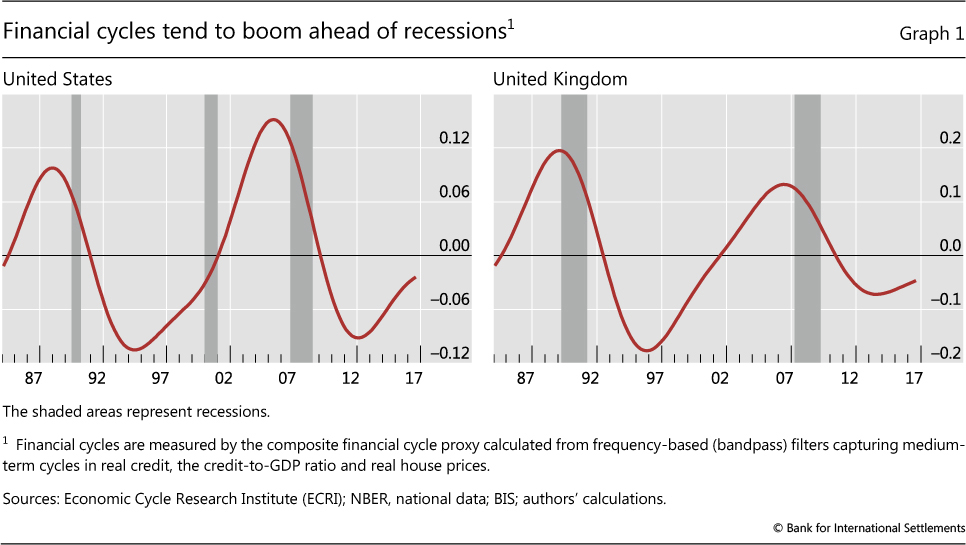
A first look at the relationship between the composite financial cycle proxy and recessions in the United States and the United Kingdom since the early 1980s illustrates these points (Graph 1). Financial cycle booms took place ahead of recessions in the early 1990s and the late 2000s. At the same time, the shallow recession in the early 2000s in the United States did not coincide with a financial cycle peak: while the economy slowed and equity prices tanked, the financial expansion continued as measured by credit and property prices, only to reverse a few years later, triggering the Great Recession. By contrast, in the United Kingdom, no recession took place in the early 2000s, so that the two recessions coincided with the two financial cycle peaks.
Why has the amplitude of financial cycles grown since the early 1980s, raising their importance for economic activity? The reasons are not yet fully understood, but arguably changes in policy regimes may be partly responsible.
Three such changes deserve particular attention. First, financial markets were liberalised starting around that time. Without sufficient prudential safeguards, this change likely allowed greater scope for the self-reinforcing interactions at the heart of the financial cycle to play out. Second, starting roughly at the same time, inflation-focused monetary regimes became the norm. And the evolving thinking of central banks led them to gradually downplay the role of monetary and credit aggregates. This meant that central banks had little reason to tighten policy if inflation remained low, even as financial imbalances built up. Finally, from the 1990s on, the entry of China and former Communist countries into the world economy, alongside the international integration of product markets and technological advances, boosted global supply and strengthened competitive pressures. Coupled with greater central bank credibility, this arguably made it more likely that inflationary pressures would remain muted even as expansions gathered pace. It also meant that financial booms could build up further and that a turn in the financial cycle, rather than rising inflation and the consequent monetary tightening, might trigger an economic downturn.9
These factors were in evidence in the run-up to the Great Financial Crisis. In many countries, short-term output volatility as well as the level and volatility of inflation fell and remained low (the so-called Great Moderation). At the same time, leverage in the financial and non-financial sectors rose. When the financial cycle turned, financial stress emerged and economies worldwide experienced a serious recession.
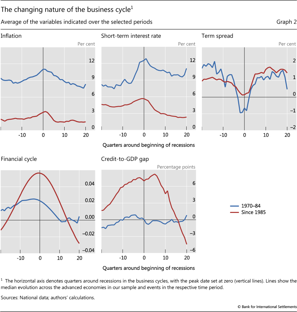
The shift in the nature of recessions is apparent when one takes a long-term cross-country perspective.10 Graph 2 documents the behaviour of key variables in the five years around business cycle turning points in our sample of 16 advanced economies (vertical lines). In the period 1970-84 (blue lines), inflation and the short-term interest rate tended to increase by several percentage points ahead of cyclical peaks and term spreads tended to plunge and become highly negative (upper panels). At the same time, there was little sign of a financial boom, whether measured by the composite financial cycle proxy or just the behaviour of credit in relation to GDP (lower panels). By contrast, since 1985 (red lines), inflation has been lower and remarkably stable around business cycle peaks, the short-term interest rate has increased only modestly and the term spread has narrowed far less. Correspondingly, strong financial cycle expansions have been very much in evidence. One could say that there has been a shift from inflation-induced11 to financial cycle-induced recessions.
Methodology
The previous graphical evidence is highly suggestive of the information that financial cycle proxies can convey about recession risk. We now perform a more systematic analysis. This calls for a number of steps.
The first step is to define the variable to be predicted. Here we follow the most widely used procedure. We take the recession dates from the National Bureau of Economic Research (NBER) or the Economic Cycle Research Institute. These rely on expert judgment based on the behaviour of several variables, such as output and employment. When such recession dates are not available, we rely on a standard business cycle-dating algorithm that identifies peaks and troughs in real GDP (Harding and Pagan (2002)). We do not consider degrees of intensity: either a recession occurs (R=1) or it does not (R=0). This, of course, means that countries with, on average, higher trend growth rates may experience fewer recessions but as many and equally sizeable slowdowns in growth. This is less of an issue for advanced economies.
The second step is to link different explanatory variables to recessions. Again, we follow a standard approach. We run a panel probit model with our recession indicator on the left-hand side, potential explanatory variables on the right-hand side and a cumulative normal distribution (Φ) describing their relationship. The model produces a probability of a recession based on the information these variables convey. Specifically, we estimate:

with single or multiple explanatory variables Xi,t for country i at time t, and different horizons (h) of one, two and three years. The estimation results give an indication of whether the explanatory variables are statistically significant in influencing the recession probability.
The final step is to judge forecast performance. Here we calculate several measures, although in the main text we rely on the area under the receiver operating characteristic (ROC) curve (Berge and Jordà (2011)). This curve maps out all possible combinations of type I errors (missed recessions) and type II errors (false alarms). The area under this curve (AUC) provides a convenient and easily interpretable summary measure of the indicator's signalling quality.12 A completely uninformative indicator has an AUC of 0.5; a perfect one an AUC of 1. The AUC of an informative indicator falls in between and is statistically different from 0.5. To ensure comparability with the existing literature, we also report other standard measures, such as the mean absolute error (MAE), the root mean square error (RMSE) and the log probability score (LPS) (eg Rudebusch and Williams (2009)). As the main insights do not change, we report these in the Online Annex.
The three variables considered - the composite financial cycle,13 the debt service ratio (DSR)14 and the term spread (the difference between the 10-year government bond rate and the three-month money market rate) - differ in terms of levels and volatility across countries.15 We thus standardise them by their mean and standard deviation.16
For the main analysis, we use quarterly data for 16 advanced economies from 1985 to 2017.17 We start at the earliest in 1985 given that, as noted, financial cycles have become more prominent since then. And, when all variables are available, we use a homogeneous panel.
To assess the validity of the results more generally, we also look at quarterly data for nine EMEs.18 Data start at the earliest in 1996 but more often around 2000. One limiting factor is that government bond markets are less developed before then, constraining the sample for the term spread. In addition, property prices are scarcer for earlier dates, limiting the ability to compute the composite financial cycle proxy. In the case of EMEs, therefore, we do not use a homogeneous panel.19 While we still show results for the composite financial cycle proxy for comparability reasons, these should be treated as indicative given the short time series.
We perform both in-sample and out-of-sample exercises. The in-sample estimation sheds light on the tightness of the lead-lag link between the variables and recessions with the benefit of hindsight (ex post); the out-of-sample analysis evaluates their performance in real time, ie taking into account only the information available up to that point. The latter is a more stringent and useful test, since it replicates the information available to policymakers when they form a judgment of the risks. Because of data limitations, we limit the out-of-sample exercise to advanced economies.
In-sample results
The in-sample results confirm that financial cycle measures provide valuable information for assessing recession risk.
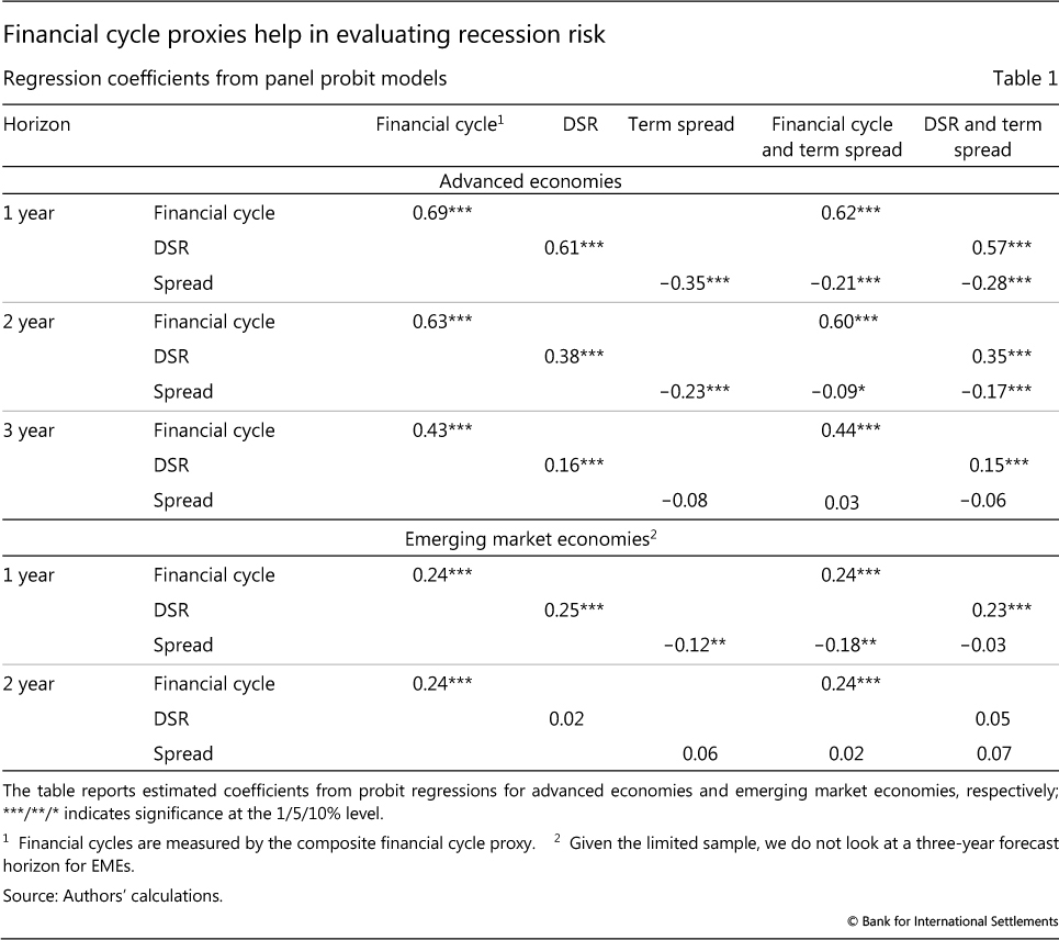
This conclusion is evident for advanced economies, for which a richer sample is available. And this is so regardless of the forecasting horizon. Coefficients for the composite financial cycle measure or the debt service burden are always highly statistically significant (Table 1, first two columns).20 AUCs underscore this message. For a one-year horizon, the AUCs of both variables are around 0.75 (Graph 3, left-hand panel, red and blue bars). For longer horizons, they decrease for the debt service burden, even though the AUCs remain significantly above the value for an uninformative variable (0.5). But the AUC of the composite financial cycle indicator remains significant and close to 0.7 at the three-year horizon, pointing to the slow-moving nature of this indicator.
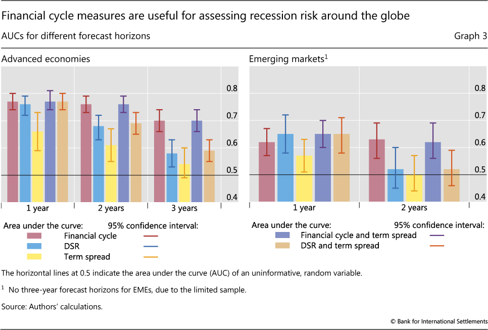
In comparison, the term spread seems to be useful only for evaluating recession risk one and two years ahead. The coefficients and AUCs are not statistically significant at the three-year horizon (Table 1, third column, and Graph 3, yellow bars).
Moreover, even at one- and two-year horizons, the composite financial cycle and debt service ratio outperform the term spread. Their AUCs are higher and the difference is statistically significant.
That said, the financial cycle proxies and the term spread seem to provide complementary information. When they are included jointly in a probit model, they all remain statistically significant up to a two-year horizon. Accordingly, AUCs and other evaluation metrics improve (Table 1, fourth and fifth columns, and Graph 3, purple and tan bars). The improvement, though, is not statistically significant. And at the three-year horizon, the gain is negligible.
The generally weaker performance of the term spread may come as a surprise. One reason is that the literature typically assesses performance at a one-year horizon or less. A second reason is that we use a panel structure, allowing for the estimation of the relevant effects across many countries. While the variables are normalised, the term spread is also affected by credit risk premia for several countries in our sample. As a result, in some episodes, the yield curve steepened rather than flattened ahead of recessions, as was the case for some periphery countries ahead of the 2011-12 euro sovereign debt crisis.21 But, more importantly, the result likely reflects the changing nature of the business cycle discussed above, in which monetary policy tightening has played a smaller role in triggering recessions and the financial cycle has gained prominence (Graph 2).
The strong performance of the financial cycle proxies is all the more remarkable given that the methodology stacks the deck against finding significant predictive power. Since the financial cycle tends to be longer than the business cycle, we cannot expect booms to precede all recessions; there will be misses. And because the financial cycle builds up and recedes slowly (see eg Graph 1), it is likely to sound several "false alarms" before and after the recession has ended. Hence, from the start, the benchmark for the AUC cannot be expected to be 1, ie the AUC of the perfect indicator.
The results for EMEs broadly mirror those for advanced economies. Both financial cycle proxies are informative, albeit less so than in advanced economies. Coefficients and AUCs for the composite financial cycle are always statistically significant, regardless of forecast horizon. The debt service ratio yields the highest AUC at the one-year horizon, although it is not significant at the two-year horizon (Table 1, second column and Graph 3, right-hand panel). Despite less developed bond markets, term spreads also seem to provide some valuable information at the one-year horizon (Table 1, third column).
Out-of-sample results
We perform two exercises to assess the indicators' performance in real time: we examine first the effect of real-time data, and then the combined effect of real-time data and model parameters estimated recursively, ie by adding one observation at a time.
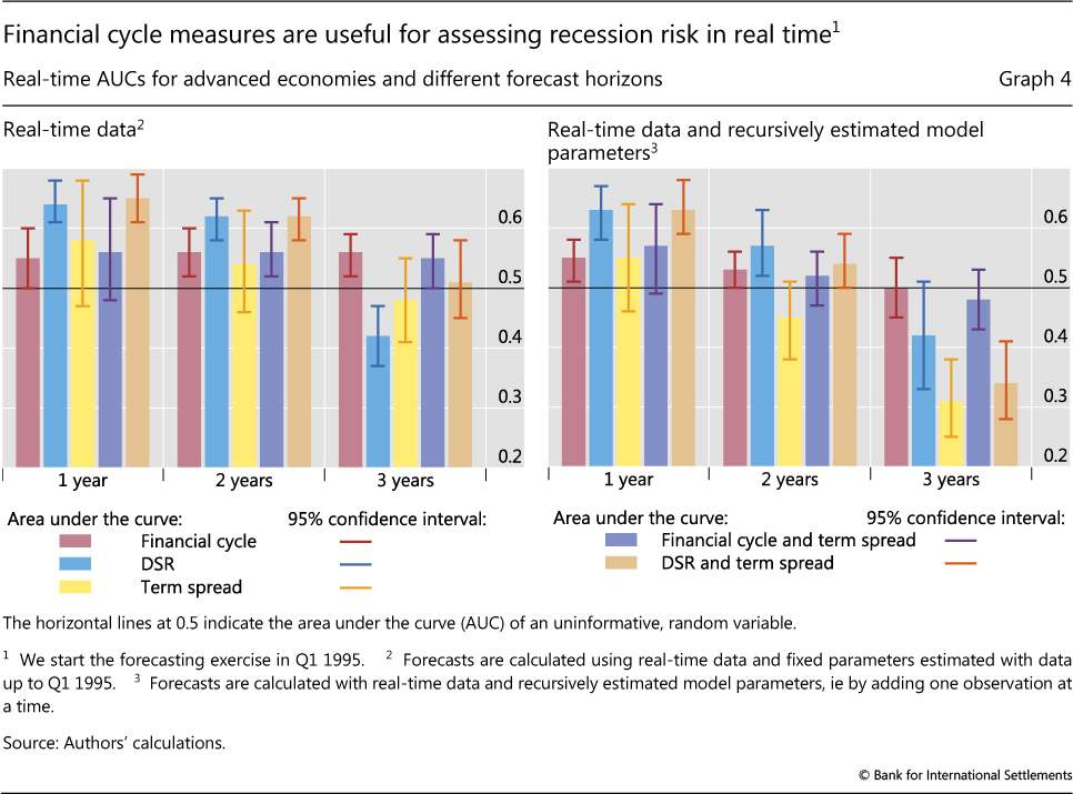
By real-time data, we mean variables normalised by the sample available at that point in time.22 Specifically, for each quarter we calculate the various financial cycle proxies with information up to that quarter and normalise them accordingly. As small samples will affect the normalisation, we exclude the first 10 years of data and start the forecasting exercise in Q1 1995. Then, to assess the impact of real-time data only, we estimate the models up to Q1 1995 and keep the parameters fixed when forecasting. And to assess the combined effect of real-time data and time-varying model parameters, we re-estimate the models every period a forecast is made (again starting from Q1 1995) and use the resulting coefficients.
Even using real-time data, financial cycle proxies provide valuable information for recession risk, and tend to outperform the term spread (Graph 4). Naturally, forecast performance drops relative to the full-sample results. But the AUC of the debt service ratio is above 0.6 up to the two-year horizon (left-hand panel). While AUCs for the composite financial cycle are lower than in the full-sample estimation, their performance is still statistically significant. In contrast, the AUCs of the term spread are not statistically significant: the signal is statistically indistinguishable from that of an uninformative indicator.
Allowing for changes in model parameters does not alter the broad message (Graph 4, right-hand panel). Both financial cycle proxies deliver AUCs that are statistically higher than 0.5 up to a two-year horizon, although not beyond. In comparison, AUCs from the term spread do not differ from that of a random indicator at all horizons.23
Conclusion
Business cycles may not die of old age (Rudebusch (2016)), but if financial booms develop, they become more fragile. This is the case in both advanced economies and EMEs. Moreover, given that financial cycles build up slowly, the corresponding proxies provide information about recession risk even at a three-year horizon. And when we run a horse race against the term spread - the indicator most widely used to assess recession risk - we find that they outperform the term spread in both in-sample and out-of-sample exercises. The debt service ratio is particular effective in this aspect. These results suggest that financial cycle proxies may be another indicator that could be useful to policymakers, professional forecasters and market participants more generally.
References
Adrian, T, F Grinberg, N Liang and S Malik (2018): "The term structure of growth-at-risk", IMF Working Papers, vol 18, no 180, August.
Aikman, D, A Haldane and B Nelson (2015): "Curbing the credit cycle", The Economic Journal, vol 125, no 585, pp 1072-109.
Bank for International Settlements (BIS) (2018): Annual Economic Report.
Beaudry, P, D Galizia and F Portier (2018): "Putting the cycle back into business cycle analysis", NBER Working Papers, no 22825.
Berge, T and O Jordà (2011): "Evaluating the classification of economic activity into recessions and expansions", American Economic Journal: Macroeconomics, vol 3, no 2, pp 246-77.
Borio, C (2014): "The financial cycle and macroeconomics: what have we learnt?", Journal of Banking & Finance, vol 45, pp 182-98, August. Also available as BIS Working Papers, no 395, December 2012.
--- (2016): "Monetary and prudential policies at a crossroads? New challenges in the new century", BIS Working Papers, no 216, September.
Borio, C and M Drehmann (2009): "Assessing the risk of banking crises - revisited", BIS Quarterly Review, March, pp 29-46.
Borio, C and P Lowe (2002): "Asset prices, financial and monetary stability: exploring the nexus", BIS Working Papers, no 114, July.
Christiansen, C, J Eriksen and S Møller (2017): "Metro Area common house price declines and US recessions", September.
Claessens, S, M Kose, and M Terrones (2012): "How do business and financial cycles interact?", Journal of International Economics, vol 87, no 1, pp 178-90.
Claessens, S and M Kose (2018): "Frontiers of macrofinancial linkages", BIS Papers, no 95, January.
Dembiermont, C, M Scatigna, R Szemere and B Tissot (2015): "A new database on general government debt", BIS Quarterly Review, September, pp 69-87.
Detken, C, O Weeken, L Alessi, D Bonfim, M Boucinha, C Castro, S Frontczak, G Giordana, J Giese, N Jahn, J Kakes, B Klaus, J-H Lang, N Puzanova and P Welz (2014): "Operationalising the countercyclical capital buffer: Indicator selection, threshold identification and calibration options", European Systemic Risk Board, Occasional Papers, no 5.
Drehmann, M, C Borio and K Tsatsaronis (2012): "Characterising the financial cycle: don't lose sight of the medium term!", BIS Working Papers, no 380, June.
Drehmann, M, M Juselius, and A Korinek (2018): "Going with the flows: new borrowing, debt service and the transmission of credit booms", NBER Working Papers, no 24549.
Eichengreen, B and K Mitchener (2003): "The Great Depression as a credit boom gone wrong", in S Wolcott and C Hanes (eds), Research in Economic History, vol 22, Emerald Group Publishing Limited, pp 183-237.
Estrella, A and F Mishkin (1998): "Predicting US recessions: Financial variables as leading indicators", Review of Economics and Statistics, vol 80, no 1, pp 45-61.
Filardo, A, M Lombardi, and M Raczko (2018): "Measuring financial cycle time", BIS Working Papers, no 755.
Guender, A (2018): "Credit prices vs. credit quantities as predictors of economic activity in Europe: Which tell a better story?", Journal of Macroeconomics, no 57, pp 380-99.
Harding, D and A Pagan (2002): "Dissecting the cycle: a methodological investigation", Journal of Monetary Economics, vol 49, no 2, pp 365-81.
Hofmann, B and G Peersman (2017): "Is there a debt service channel of monetary transmission?", BIS Quarterly Review, December, pp 23-37.
Huffman, W and J Lothian (1984): "The gold standard and the transmission of business cycles, 1833-1932", in D Bordo and A Schwartz (eds), A retrospective on the classical gold standard, NBER, pp 1821-931.
Juselius, M and M Drehmann (2015): "Leverage dynamics and the real burden of debt", BIS Working Papers, no 501, May.
Liu, W and E Moench (2016): "What predicts US recessions?", International Journal of Forecasting, vol 32, no 4, pp 1138-50.
Lombardi, M, M Madhusudan and I Shim (2017): "The real effects of household debt in the short and long run", BIS Working Papers, no 607, January.
Mian, A, A Sufi and E Verner (2017): "Household debt and business cycles worldwide", The Quarterly Journal of Economics, vol 132, no 4, pp 1755-817.
Ponka, H (2017): "The role of credit in predicting US recessions", Journal of Forecasting, vol 36, no 5, pp 469-82.
Rudebusch, G (2016): "Will the economic recovery die of old age?", Federal Reserve Bank of San Francisco, Economic Letters, February.
Rudebusch, G and J Williams (2009): "Forecasting recessions: the puzzle of the enduring power of the yield curve", Journal of Business and Economic Statistics, vol 27, no 4, pp 492-503.
Schularick, M and A Taylor (2012): "Credit booms gone bust: Monetary policy, leverage cycles, and financial crises, 1870-2008", American Economic Review, vol 102, no 2, pp 1029-61.
Zarnowitz, V (1999): "Theory and history behind business cycles: are the 1990s the onset of a golden age?", Journal of Economic Perspectives, vol 13, no 2, pp 69-90.
1 The authors would like to thank Stijn Claessens, Ben Cohen, Mikael Juselius, Marco Lombardi, Hyun Song Shin and Kostas Tsatsaronis for helpful comments and Anamaria Illes for excellent research assistance. The views expressed in this article are those of the authors and do not necessarily reflect those of the BIS.
2 See Claessens and Kose (2018) for a literature review on research exploring macro-financial linkages.
3 Recent papers making use of financial expansion-related variables, such as financial intermediary balance sheet conditions, property prices, credit growth or credit spreads, include Liu and Moench (2016), Christiansen et al (2017), Ponka (2017) and Guender (2018). All these papers base their analysis on US data only, with the exception of Guender (2018), who instead looks at a set of European countries.
4 Additional analysis (not shown) indicates that the financial cycle measures are also valuable in assessing recession risk when considering exclusively the United States, which has been the focus of the literature. For this country, the proxies do as well as the spread. Given that we use data from 1985, however, this comparison is based on only three recessions.
5 See also Juselius and Drehmann (2015) for a description of the financial cycle in terms of the joint behaviour of leverage - approximated by the ratio of debt to assets - and the debt service ratio.
6 See also Hofmann and Peersman (2017).
7 See eg Aikman et al (2015), Claessens et al (2012) or Drehmann et al (2012).
8 For instance, Filardo et al (2018) document the time-varying nature of financial cycles and explore underlying drivers. There is also some evidence that business cycles have become longer in recent years (eg Beaudry et al (2018)).
9 For a discussion of changes in policy regimes and their implications for monetary and financial stability, see eg Borio and Lowe (2002) and Borio (2016).
10 Interestingly, the recessions since the early 1980s have come to resemble those that were the norm under the pre-WWI classical gold standard (eg Huffman and Lothian (1984)) and in the run-up to the Great Depression in the 1920s (Eichengreen and Mitchener (2003)). This was the previous globalisation era; like today's, it was also characterised by price stability and a high degree of both trade and financial integration. See BIS (2018), Chapter 1.
11 Zarnowitz (1999) uses the term "central bank recession" to refer to the common view that recessions are always driven by monetary policy tightening.
12 A probability can be transformed into a binary indicator, which is equal to 1 ("on") if it is above a critical threshold T, and zero ("off") otherwise. A type I error (missed call) occurs if the binary indicator is "off" but a recession follows; and a type II error (false alarm) if it is "on" but no recession follows. By changing the critical threshold T, the fraction of type I and type II errors changes. Technically, there is no direct mapping between the significance of coefficients in the probit equation and the AUC, especially if the probit includes more than one variable. In that case, the probit regression coefficients may be statistically significant, even if their inclusion does not change the AUC much.
13 Drehmann et al (2012) use bandpass filters with frequencies from eight to 32 years to extract medium-term cyclical fluctuations in real (inflation-adjusted) credit, the credit-to-GDP ratio and real property prices, which they then average to derive a composite measure of the financial cycle. We modify the approach slightly by applying the filter directly to the log-level of the individual series instead of filtering the growth rates. The data on total credit, credit-to-GDP ratios and long-run property prices are taken from BIS statistics.
14 While not shown explicitly, results based on other individual financial cycle proxies, such as the deviation of the credit-to-GDP ratio from its long-term trend ("credit gap") or a similar normalisation for property prices ("property price gap") yield broadly similar results.
15 Data on debt service ratios are published on the BIS website (Dembiermont et al (2015)) from 1999. We extend them backwards using the same methodology but rely on country-specific proxies to backdate the input data in several cases.
16 This has the additional benefit of implicitly controlling for fixed effects in a similar way to Chamberlain's random effects probit model.
17 The countries included are Australia, Belgium*, Canada, Finland*, France, Germany, Ireland*, Italy, Japan, the Netherlands*, Norway*, Spain, Sweden, Switzerland, the United Kingdom and the United States. For countries denoted with *, we date business cycles with a business cycle-dating algorithm.
18 EMEs included are Brazil, the Czech Republic, Hungary, Korea, Malaysia, Poland, Russia, South Africa and Thailand. For these countries, we always date business cycles with a business cycle-dating algorithm. For an EME to be included, we require that all three variables are available and that we have at least 10 years of spread and debt service ratio data. In addition, we also only include an EME if we observe at least one recession in the sample.
19 The sample is homogeneous for regressions with the debt service ratio and the term spread.
20 We obtain standard errors by block bootstrapping in order to account for cross-country correlations.
21 When we remove the euro area periphery countries (ie Ireland, Italy and Spain), AUCs for the term spread increase to 0.71 and 0.65 at the one- and two-year horizons, respectively, while the information content of the financial cycle proxies is little affected.
22 For the data, we would ideally use real-time releases. However, these are not available for the panel, so we use quasi-real-time information, ie we take the latest data vintage and calculate the financial cycle and normalise the variable using data only up to that point.
23 Allowing parameter estimates to vary as the sample is increased seems to reduce forecast accuracy to some extent: the AUCs obtained when parameters are fixed are slightly higher.