Term premia: models and some stylised facts

We review methods and models for estimating term premia on long-term government bonds. We then use these models to estimate term premia on US and euro area bonds and explore their recent behaviour. Although the models produce different estimates for the level of term premia, they largely concur on the trends and dynamics. While low (and sometimes negative) term premia have helped to keep yields unusually low, recent yield movements have tended to reflect shifts in expected short-term rates rather than in the premia. We find that co-movements in real term premia (rather than inflation risk premia or expected rates) have contributed to co-movements between yields in the United States and the euro area.¹

JEL classification: G10, G12.

Yields on long-dated bonds are made up of two parts: the returns expected from comparable, shorter-dated instruments over the same time period, and an additional component, or term premium. This term premium is normally thought of as the extra return (a risk premium) that investors demand to compensate them for the risk associated with a long-term bond. But it may also be influenced by supply and demand imbalances for a specific instrument, or several other factors. Typically, expected interest rates and term premia are extracted using models based on a small number of risk factors, under the assumption that consistency is maintained between yields at different maturities through the absence of arbitrage opportunities. The models are estimated from market data, in some cases supplemented by survey data and macroeconomic indicators.

In this Special Feature, we examine some methods and models used to distinguish these different bond yield components. We focus on benchmark government bonds for the United States and the euro area. Both of the corresponding yield curves benefit from deep, liquid markets with a broad range of maturities, and act as benchmarks for the pricing of many other assets worldwide.

We then make use of this decomposition to study recent drivers of US and euro area yields. In recent years, government bond yields have not always responded predictably to macroeconomic or monetary policy news. Long-term yields in the United States remained stubbornly low even as the Federal Reserve initiated a series of interest rate hikes away from zero starting in late 2015. From mid-2016, as growth prospects have picked up, yields in both the United States and in Europe have trended higher, but long-term yields have not always kept up with those at the short-term end. Analysts have debated the causes and implications of a flat, or even downwards-sloping, term structure at a time of broadly robust growth.

The various models we study give different estimates for the levels of estimated term premia, but they tend to agree on the general trend and dynamics. In particular, all estimates point to an overall downward trend in term premia both in the United States and in the euro area since the 2007-09 Great Financial Crisis (GFC). Premia have increased somewhat recently, but are still well below pre-GFC levels. The models also tend to find that premia are highly correlated across currencies, while interest rate expectations are not. Changes in rate expectations, especially for real (inflation-adjusted) interest rates, have driven yields at times, including those of US Treasuries in the last year or two. But low term premia have also contributed to the recent puzzling behaviour in yields and the term structure, including through international spillovers.

The first section discusses the basics of term premia models and explores how they are used to separate the various components of market yields. The second and third apply these insights to benchmark 10-year government bond yields in the United States and the euro area. The fourth asks what correlations across the different estimated components can tell us about the drivers of US and euro area rates. The last section concludes.

Methods for estimating term premia

As mentioned above, long-term interest rates can be broken out into a part that reflects the expected path of short-term interest rates and a term premium.² In standard finance theories, the latter part represents the compensation, or risk premium, that risk-averse investors demand for holding long-term bonds. This compensation arises because the return earned over the short term from holding a long-term bond is risky, whereas it is certain in the short term for a bond that matures over the same short investment horizon. While some types of investor, such as pension funds, may consider long-term bonds less risky given their long-term liabilities, most other investors would tend to view them as more risky.

More generally, though, the term premium would reflect this type of compensation for risk only if markets were perfectly functioning and frictionless. In reality, a number of other influences may affect bond yields, and thus the estimated expectations and term premium components. One such influence is supply-demand imbalances, such as those brought on by outsize official sector purchases of government bonds in recent years. Such effects may be compounded by burgeoning demand for long-term bonds from insurance and pension funds, as they try to hedge duration risk, especially in an environment of falling yields (Domanski et al (2015)). Sometimes institutional factors might lead to outsize investor demand for specific maturities, creating a "preferred habitat" effect that will be reflected in term premia (Modigliani and Sutch (1966), Vayanos and Vila (2009)).

One simple way of estimating the term premium is to subtract a survey measure of the average expected short rate from the observed bond yield. There are some drawbacks with this approach, however. Survey data are not updated frequently and (typically) include only a limited set of forecast horizons. Surveys may not always represent actual expectations of market participants, for instance because forecasters compete for business or for influence through their calls or because one or more large players have a disproportionate impact on the market.

The modern term structure literature provides an alternative way of disentangling term premia and interest rate expectations.³ The starting point is the assumption that bonds are priced in a way that precludes arbitrage opportunities across all maturities. In other words, the pricing is assumed to make it impossible to form a portfolio consisting of bonds with different maturities that generates a riskless profit.

Typically, these models represent the time-series dynamics of bond yields with simple vector autoregressions. Restrictions are then imposed to reflect the no-arbitrage assumption across the entire maturity spectrum, giving rise to alternative, risk-neutral dynamics for yields. The differences between the actual ("objective") and the risk-adjusted dynamics reflect market participants' risk preferences. By exploiting these two dynamics, it is possible to decompose yields into expectations of future interest rates and term premia.

Much of the term structure literature has relied on models where a small set of yield-based factors is assumed to drive bond yield movements. One example is the model proposed by Adrian et al (2013, henceforth ACM), which uses principal components of bond yields as pricing factors.⁴ The factors are weighted sums of yields with weights derived through statistical techniques. These models are appealing for their simplicity. That said, the yields so derived are prone to overreacting to changes in the general level of interest rates because they rely only on yield information. In particular, they may tend to interpret a change in interest rates as evidence that the steady-state (long-run) interest rate has changed correspondingly. This leads to exaggerated movements in distant-horizon interest rate projections.

But there are alternative approaches. Precisely because term structure models try to capture the very high persistence of yields, ie their tendency to be highly correlated over time, some researchers have included interest rate survey data in the models, even as they recognise the shortcomings of such data.⁵ Kim and Wright (2005, henceforth KW) use one such model to estimate US term structure dynamics based on survey data on future three-month interest rates. Just as in the previous set of models, however, the factors driving interest rates are derived only from interest rates themselves.

Other models include macroeconomic factors in addition to, or instead of, yield factors. These macroeconomic factors are motivated by what investors are likely to care about when pricing bonds. Typically, they include inflation and some measure of economic activity.⁶ Whatever the choice of factors used, these typically also represent the risk factors in the pricing model, ie the factors that determine the size and the dynamics of risk premia. An example of such a model is the one used by Hördahl and Tristani (2014, henceforth HT), which includes data on nominal and real (index-linked) yields, inflation, and a measure of economic slack ("output gap"), as well as survey data on future short-term interest rates and future inflation rates.

With more data and assumptions, we can obtain still more detail about the components of long-term yields. Specifically, we can split the term premium into two parts: a real risk premium - the compensation required to bear risk associated with variable future short-term real interest rates - and an inflation risk premium, which is related to uncertain future inflation developments.⁷ And one can separate the expectations component into a part that reflects average expected future short-term real interest rates, and another that captures expected average inflation until the bond matures.

As with any estimation exercise, there are important caveats. For one thing, all term premia estimates are model-dependent, and also subject to parameter uncertainty. Second, previously estimated term premia will change over time as the model parameters are updated, insofar as the most complete and up-to-date information is seen as useful in capturing earlier developments in model-implied expectations and premia. Third, macro data revisions will lead to changes in estimates based on models that use macro data. In some cases, such as with potential output series that are used to calculate the output gap, revisions can at times be substantial. Revisions of estimates therefore complicate the real-time performance of these models. And models that rely on unobserved variables such as the output gap are sensitive to the estimation of those variables, for instance, the measurement of trends as more data become available.

Moreover, any model should be seen as a useful simplifying tool, but one that does not necessarily capture various real-life influences. An example of the latter is the recent experience with policy rates stuck at the zero lower bound (ZLB) or, in some cases, below zero (see eg Wu and Xia (2016, 2018)). For a number of reasons, zero or negative interest rates are likely to behave differently from positive ones. Models that do not explicitly take into account the probability of hitting the ZLB are good approximations when interest rates are far away from it. But, when interest rates are close to it, such models might generate interest rate forecasts below the bound as well as biased term premia estimates.

US term premia estimates and recent developments

We start off by comparing estimates of term premia on 10-year US Treasury bonds obtained from the three term structure models discussed above. These are the ACM yield-factor-only model, the KW yield-factor model with additional information from surveys, and the HT macro-finance factor model that also includes survey information.

Graph 1 plots the premia estimates from each of these models. The left-hand panel also plots a model-free alternative estimate, calculated as the 10-year yield minus the corresponding 10-year average short-rate expectation, as reported once a year by the Survey of Professional Forecasters (SPF).

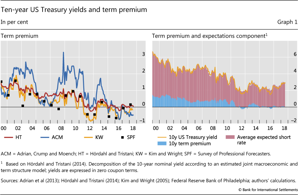
The graph illustrates how different methods can generate different levels of the term premia. Estimates derived from the ACM and the HT models can differ by as much as 200 bps. The discrepancy partly reflects the assumptions embedded in these estimates, as discussed above.⁸

Nonetheless, these models broadly agree on the trends and dynamics of premia. All estimates suggest a general downward trend since the GFC. The trend accounts for a large share of the overall evolution in the 10-year yield (Graph 1, right-hand panel). All the models would agree that rising 10-year US Treasury yields in 2017-18 largely reflect an increase in the expected short rate over the subsequent 10 years. Correlations of monthly changes in premia estimates from different pairs of models range from 0.77 to 0.92.

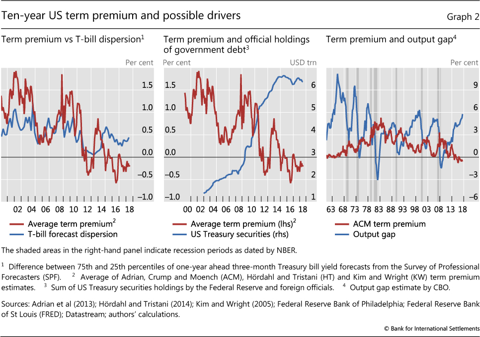
What might explain the fall in term premia since the GFC? Two potential contributing factors could be declining uncertainty about the projected path of short rates, and demand pressures from central banks and other price-inelastic purchasers of Treasuries.

The general decline in the term premium during 2009-13 coincided with a smaller dispersion of survey expectations about future rates (Graph 2, left-hand panel). This reduced uncertainty may reflect forward guidance and other Fed communications policies. The fall in dispersion may also have reflected the smaller distance of short-term rates from zero, combined with the perception (reinforced by the Fed's forward guidance) that any rate increases were unlikely in the near term.⁹ This pattern ended around the time of the 2013 "taper tantrum", when comments from Fed officials led the market to expect an imminent removal of monetary accommodation.

Purchases by the Fed and by the official sector outside the United States also played a role. The post-GFC downward trend in the term premium coincided with a sharp rise in the Fed's and foreign official holdings of Treasuries, in line with the notion that demand pressures from these sources helped to push down yields (Graph 2, centre panel).

In addition, the downward trend of the term premium in the decade since the GFC may have been linked to the more appealing risk properties of bonds. Specifically, bond yields tended to fall in response to any sign of setbacks in the economic recovery as investors raised their expectations of further monetary stimulus or pushed back the expected start of policy normalisation. As often happens after a severe crisis, awareness of "tail risks" rose, and with it the desire to insure against such risks. Hence, in the GFC's aftermath, bonds took on some insurance-like properties. As a result, investors may have been willing to hold bonds even as the term premium fell towards zero or became negative. The resulting flight to safety boosted the demand for safe assets. Tighter regulatory requirements may also have played a role, such as for banks' holdings of liquid assets or collateralisation of derivatives positions.

We can uncover some further general properties of term premia when we look over a longer time span. For one thing, term premia are normally countercyclical - although, as discussed above, tail risk concerns helped keep term premia low after the GFC. In other words, they tend to rise when output is below potential or the economy is in recession, as investors seek higher compensation for being exposed to interest rate risk in bad times (Graph 2, right-hand panel). The fall in term premia during the current recovery represents a return to this pattern. And near-zero term premia are not unprecedented: for much of the 1960s, the premium hovered just above zero. From 1961 to 2018, however, the average according to the ACM model (which can be estimated over the longest time period) was around 160 basis points.

In addition to term premia, each modelling approach produces estimates of average expected short-term interest rate over any given horizon. All four measures discussed above show falling 10-year average expected short rates after the GFC (Graph 3, left-hand panel). The ACM model, which relies exclusively on yield information, displays a sharper initial decline, followed by an earlier rise. All four measures agree that the average expected short rate increased in 2017 and 2018.

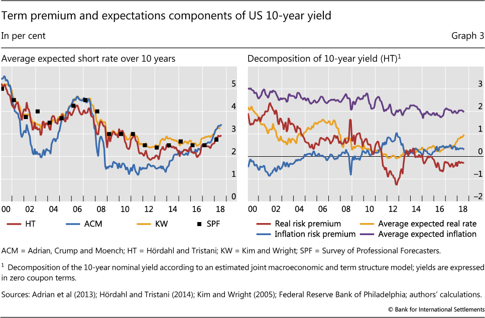
When we decompose the US 10-year yield further into real and inflation-linked components, we find that much of the initial decline in long-term yields during and after the GFC was due to a sharp drop in average expected real interest rates as the crisis unfolded. This was followed by a more gradual decline in expected real rates during the great recession that followed (Graph 3, right-hand panel). This observation is in line with the notion that investors' perception of the natural rate of interest may have fallen significantly during this time. Moreover, although the real risk premium remained elevated during and immediately after the Lehman collapse, it declined sharply as the Fed progressively eased monetary policy via unconventional measures. The decomposition also suggests that much of the rise in long-term yields in 2017-18 has been due to higher expected future real interest rates. By contrast, expected future inflation, the real risk premium and the inflation risk premium have changed little, with the real risk premium remaining unusually low.

Euro area estimates and recent developments

Similar to US Treasury yields, the euro area's benchmark long-term government bond yields declined more or less steadily during the GFC and its aftermath.¹⁰ However, in 2014, euro area yields started to fall more rapidly than those in the United States. This was largely due to the market's anticipation of the ECB's asset-buying Public Sector Purchase Programme (PSPP) and its subsequent implementation (from early 2015). With a brief interruption, when they jumped in May-June 2015,¹¹ euro area yields continued to decline until the second half of 2016. Since then they have risen only modestly, even as US yields have increased more decisively.

To an even greater extent than for the United States, much of the decline in euro area yields up to mid-2016 reflected falling term premia (Graph 4, left-hand panel). The timing of this fall underscores the important role that supply-demand imbalances such as the ECB asset purchases (and the related market expectations) can play. Moreover, with economic growth weak, the hedging properties of core euro area sovereign bonds became particularly valuable to investors, leading them to tolerate even deeply negative term premia.

As for the United States, term premia estimates for the euro area differ depending on the model used, though they agree on the overall trend and dynamics. The centre panel of Graph 4 displays 10-year premia estimates calculated following the ACM methodology, alongside the HT model estimates and estimates from a model used by the Bank of France.¹² These estimates are less correlated than for US models. While the correlation of changes in premia between the HT and the ACM model is around 0.55, the premia estimated by the Bank of France are essentially uncorrelated with the other two. Apart from limited correlations, these estimates also differ in their overall levels. Towards the end of the sample period, the difference between the HT and ACM estimates is around 140 basis points. Since 2016, Consensus Economics has published quarterly long-term interest rate forecasts that can be used to back out model-free 10-year term premia estimates. These estimates (dots in Graph 4, centre panel) are closer to the HT premia and the Bank of France estimates, whereas the ACM estimates differ from the survey measure by around 100 basis points in recent quarters.

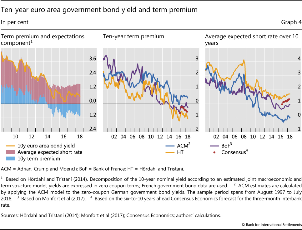
It is not clear exactly what lies behind the wide range in premium estimates across models. But one reason why the HT model tends to produce considerably lower estimates may be that it relies on an array of data types, whereas the ACM model uses only nominal yield data. As noted above, a model that relies only on yield information may be more prone to interpret the very low level of interest rates in the past few years as evidence that the steady-state interest rate level has fallen substantially due to the highly persistent nature of interest rates. The HT model, by contrast, is further disciplined by the inclusion of real yields, macroeconomic data and survey expectations. Consistent with this, as noted, the HT average expected short-term interest rate is closer to the expectations expressed by survey respondents (Graph 4, right-hand panel).

Just as in the United States, euro area term premia have been influenced by official sector asset purchases (Graph 5, left-hand panel) as well as the output gap (centre panel). A rise in official holdings likely helped to keep euro area bond yields low, but the steady (and clearly announced) pace of purchases makes it difficult to tie short-term fluctuations in the premia to these purchases. While weak macroeconomic performance may well have played a role after the GFC (for example, by pushing investors to safe assets), the steady narrowing in the euro area output gap since 2014 has been accompanied by a further drop in the term premium.

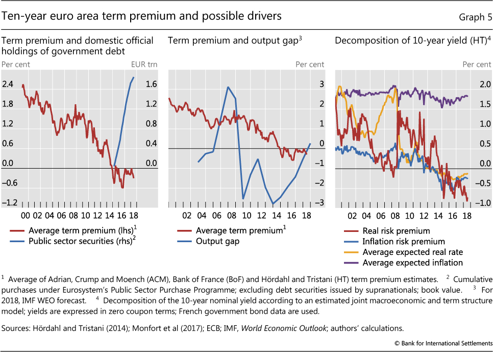
We can gain further insights into the movements of euro area bond yields by decomposing the 10-year yield into its four components (Graph 5, right-hand panel). According to the HT model, while the drop in the euro area yield during the GFC was mainly due to falling average expected real interest rates, much of the sharp drop in 2014-15 seems to have been due to a rapidly falling real term premium. In contrast to the United States, where (except for a spike in 2012) inflation risk premia were more or less stable after the GFC, the fall in euro area yields was reinforced by a drop in the inflation risk premium. In other words, insofar as the ECB PSPP placed downward pressure on yields, it did so by lowering term premia, and more so on nominal than on real bond yields. In 2017 and 2018, modest increases in expected interest rates and in the inflation risk premium component led to a moderate increase in bond yields, although a decline in the real term premium offset much of the effects of changes in the other components. For US yields, by contrast, rising expected real rates have been accompanied by relative stability in the other components and have been largely passed through into nominal yields.

Cross-country correlations

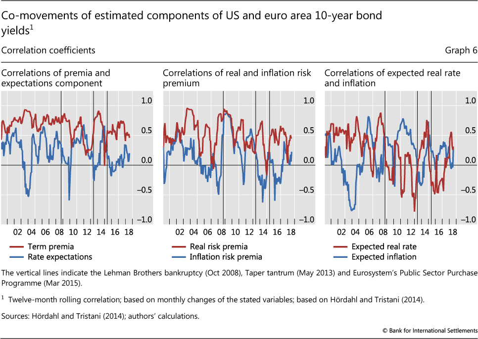
Term premia are typically highly correlated across sovereign yields in different countries, contributing to significant co-movements in the yields.¹³ Term premia in the euro area and the United States have indeed followed one another closely in recent years. The rolling one-year correlation between monthly changes in US and euro area term premia has typically hovered between 0.6 and 0.9, although it has displayed wider swings since the GFC (Graph 6, left-hand panel). In particular, the rolling correlation dropped markedly after the Lehman collapse in 2008, at the peak of the euro area sovereign debt crisis in 2012, and as the ECB launched its bond purchase programme in 2015. However, there was a clear surge in the correlation of term premia around the time of the taper tantrum in 2013, when rising global premia reflected declining global risk appetite as the outlook for US monetary policy became less certain. The high correlation is largely driven by the real components. Correlations of real risk premia tend to be much higher than those of inflation risk premia (centre panel).

Looking back further in time, US and euro area term premia typically tend to be more correlated than the respective expectations components (Graph 6, left-hand panel). Historically, the term premium correlation has generally been above 0.5, reaching at times up to 0.93. In contrast, the correlation of interest rate expectations between the United States and the euro area has fluctuated between 0 and 0.6. This correlation has even fallen below zero during some periods, including 2003-04, when the fed funds rate was lowered to a then record-low 1%; the 2013 taper tantrum; and late 2015, when the Fed made its first post-GFC rate hike, with the ECB not moving in tandem. The low correlation of interest rate expectations reflects low correlations of both expected real rates and expected inflation (Graph 6, right-hand panel).

Conclusions

Yield curve models can offer a number of insights about the drivers of movements in US and euro area benchmark yields over the past several years. The estimated term premia can differ sharply depending on the model used but, in most cases, they have trended downwards since the GFC. While low term premia have helped to keep yields low, recent yield movements have tended to reflect shifts in expected short-term rates, particularly for the United States in 2017-18. Real risk premia, rather than premia for inflation risk, appear to have generally played an important role, while expected real rates have had a greater effect on expected short rates than expected inflation has.

What drives the term premia? We have identified a number of possible factors, including uncertainty, official sector purchases, the business cycle and regulation. But the relative impact of these factors can shift over time and is very hard to measure. Moreover, other factors may also be at work. Sound estimation methods for the bond yield components are an important first step in understanding how these factors play out in bond markets and the wider economy.

References

Ang, A and M Piazzesi (2003): "A no-arbitrage vector autoregression of term structure dynamics with macroeconomic and latent variables", Journal of Monetary Economics, vol 50, no 4, pp 745-87.

Adrian, T, R Crump and E Moench (2013): "Pricing the term structure with linear regressions", Journal of Financial Economics, vol 110, no 1, pp 110-38.

Dai, Q and K Singleton (2000): "Specification analysis of affine term structure models", Journal of Finance, vol 55, no 5, pp 1943-78.

Domanski, D, H S Shin and V Sushko (2015): "The hunt for duration: not waving but drowning?", BIS Working Papers, no 519, October.

Duffie, D and R Kan (1996): "A yield-factor model of interest rates", Mathematical Finance, vol 6, pp 379-406.

Hördahl, P and O Tristani (2014): "Inflation risk premia in the euro area and the United States", International Journal of Central Banking, vol 10, no 3, pp 1-47.

Hördahl, P, O Tristani and D Vestin (2006): "A joint econometric model of macroeconomic and term structure dynamics", Journal of Econometrics, vol 131, no 1/2, pp 405-44.

Joslin, S, K Singleton and H Zhu (2011): "A new perspective on Gaussian dynamic term structure models", Review of Financial Studies, vol 24, pp 926-70.

Jotikasthira, C, A Le and C Lundblad (2015): "Why do term structures in different currencies co-move?", Journal of Financial Econometrics, vol 115, no 1, pp 58-83.

Kim, D and A Orphanides (2007): "The bond market term premium: what is it, and how can we measure it?", BIS Quarterly Review, June, pp 27-40.

--- (2012); "Term structure estimation with survey data on interest rate forecasts", Journal of Financial and Quantitative Analysis, vol 47, pp 241-72.

Kim, D and J Wright (2005): "An arbitrage-free three-factor term structure model and the recent behavior of long-term yields and distant-horizon forward rates", Finance and Economics Discussion Series, Board of Governors of the Federal Reserve System, no 2005-33, August.

Modigliani, F and R Sutch (1966): "Innovations in interest rate policy", American Economic Review, vol 56, no 1/2, pp 178-97.

Monfort, A, F Pegoraro, J-P Renne and G Roussellet (2017): "Staying at zero with affine processes: An application to term structure modelling", Journal of Econometrics, vol 201, no 2, pp 348-66.

Riordan, R and A Schrimpf (2015): "Volatility and evaporating liquidity during the bund tantrum", BIS Quarterly Review, September, pp 10-11.

Rudebusch, G and T Wu (2008): "A macro-finance model of the term structure, monetary policy, and the economy", Economic Journal, vol 118, no 530, pp 906-26.

Vayanos, D and J-L Vila (2009): "A preferred habitat model of the term structure of interest rates", NBER Working Papers, no 15487, November.

Wu, J and F Xia (2016): "Measuring the macroeconomic impact of monetary policy at the zero lower bound", Journal of Money, Credit and Banking, vol 48, no 2/3, pp 253-91.

--- (2018): "The negative interest rate policy and the yield curve", BIS Working Papers, no 703.

¹ The authors would like to thank Claudio Borio, Phurichai Rungcharoenkitkul, Hyun Song Shin and Philip Wooldridge for comments and Bilyana Bogdanova and Nicholas LeMercier for research assistance. The views expressed in this article are those of the authors and do not necessarily reflect those of the BIS.

² See also Kim and Orphanides (2007) for a review of key concepts and methods.

³ See eg Duffie and Kan (1996), Dai and Singleton (2000) and Joslin et al (2011).

⁴ In principal components analysis, a set of time series (such as bond yields of different maturities observed over time) is used to generate a second set of series (principal components), which are not correlated with (orthogonal to) each other and which, as a group, capture a large share of the variation in the original series. The first principal component usually accounts for the most variation in the underlying variables; each additional principal component allows a more accurate rendering of the original series.

⁵ See eg Kim and Orphanides (2012).

⁶ Examples include Ang and Piazzesi (2003), Hördahl et al (2006), and Rudebusch and Wu (2008).

⁷ Typically, this requires inflation data in addition to yields, in order to construct a real stochastic discount factor alongside the nominal one. Moreover, data on real (index-linked) bond yields are helpful to pin down the dynamics of real yields, but not strictly necessary. The Hördahl and Tristani (2014) model uses real yield data in addition to nominal yields, macro factors and survey information.

⁸ The discrepancies are not, however, explained by fitting errors implied by the models, as these models tend to fit the yield data very well. For example, the standard deviation of the residual between the observed 10-year yield and the corresponding yield from the HT model is below 9 basis points over the January 1981 to July 2018 sample period.

⁹ Towards the end of this period, policy rates and some bond yields did fall below zero in a few economies, including the euro area, although not in the United States.

¹⁰ Benchmark government bond yields in the euro area are often proxied by government bond yields in France or Germany, as the credit risk of these bonds is deemed to be negligible.

¹¹ This episode corresponded to a short-lived deterioration in market liquidity. See Riordan and Schrimpf (2015).

¹² These models make use of different euro area benchmark rates: the HT model uses 10-year French government bond yields, the ACM model 10-year German government bond yields and the Bank of France 10-year OIS rates on EONIA. However, these benchmark rates are very close to each other, with an average absolute difference of around 25 basis points.

¹³ See eg Jotikasthira et al (2015).