Wealth inequality and monetary policy
This feature explores the recent evolution of household wealth inequality in advanced economies by looking at valuation effects on household assets and liabilities. Using household survey data, we analyse the possible drivers of wealth inequality and the potential effect of monetary policy through its impact on interest rates and asset prices. Our simulation suggests that wealth inequality has risen since the Great Financial Crisis. While low interest rates and rising bond prices have had a negligible impact on wealth inequality, rising equity prices have been a key driver of inequality. A recovery in house prices has only partly offset this effect. Abstracting from general equilibrium effects on savings, borrowing and human wealth, this suggests that monetary policy may have added to inequality to the extent that it has boosted equity prices.1
JEL classification: D31, E52.
Inequality is back in the international economic policy debate. Evidence of a growing dispersion of income and wealth within major advanced and emerging market economies (EMEs) has sparked discussions about its economic consequences. Although there is no consensus on the relationship between inequality and growth, there are concerns that rising inequality may become a serious economic headwind.
While traditionally considered to be of secondary importance, questions about the possible distributional effects of monetary policy have recently come to the fore. Unprecedented monetary accommodation since the onset of the Great Financial Crisis (GFC) has given rise to concerns that monetary policy may have been contributing to inequality (Cohan (2014) and Wolf (2014)).
At least two arguments support the view that unconventional monetary policy may have had a larger than usual effect on the distribution of wealth - which we define as assets net of liabilities - across households. First, the short end of the yield curve has been at zero and the long end has been compressed for a long time. This suggests large and persistent valuation effects on financial assets. Second, some unconventional policy measures have explicitly targeted asset prices. As a result, the distributional effects of recent policy actions have attracted the attention of the general public, drawing central banks into the debate on inequality, as highlighted by several recent speeches by top monetary policymakers (Yellen (2015), Draghi (2015), Mersch (2014) and Haldane (2014)).
This special feature explores the evolution of wealth inequality since the GFC and the possible role of monetary policy. The next section analyses the evolution of wealth inequality around the crisis, focusing on the role of valuation effects from interest rate and asset price changes. The following section considers the role of monetary policy as a possible driver.
Wealth inequality since the Great Financial Crisis: a simulation
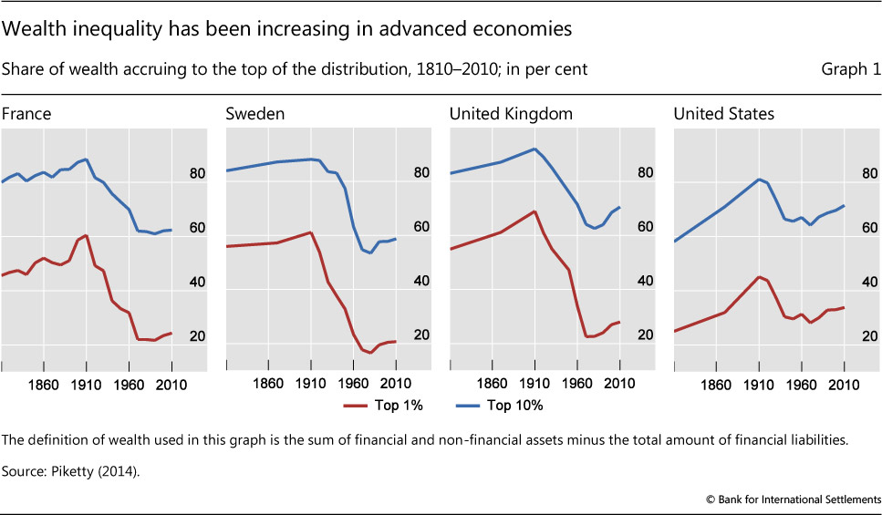
Wealth inequality has been rising in advanced economies (AEs) (Graph 1). Data available from 1810 to 2010 suggest that, as measured by the share of the top 1% of the wealth distribution, inequality has been increasing since the 1980s. While inequality remains below the levels prevailing in the second half of the 19th century, this rise marks the end of a trend of declining inequality that lasted for most of the 20th century.2
Wealth inequality has been increasing in tandem with income inequality (see the discussion in Box 1). Indeed, one popular explanation for the rise in wealth inequality is a "snowball effect" from rising income inequality. To the extent that those at the top of the income distribution save a larger fraction of their incomes, higher income inequality adds to the concentration of wealth. In turn, for given returns on capital and labour, wealth concentration exacerbates income inequality (Saez and Zucman (2014)).
It is important to note at the outset that any assessment of trends in inequality suffers from serious data limitations. Typically, the data come from household expenditure surveys in which the top of the distribution tends to be underrepresented, especially with respect to wealth. To account for dynamics at the top, researchers have begun to use tax return data (eg Saez and Zucman (2014) and Alvaredo et al (2015)). Even so, tax avoidance and evasion may induce a downward bias in estimates of income and wealth at the top.
Box 1
Trends and drivers of income inequality
The recent debate has focused mostly on income inequality - the distribution of returns from labour and capital - within, but also across, countries.
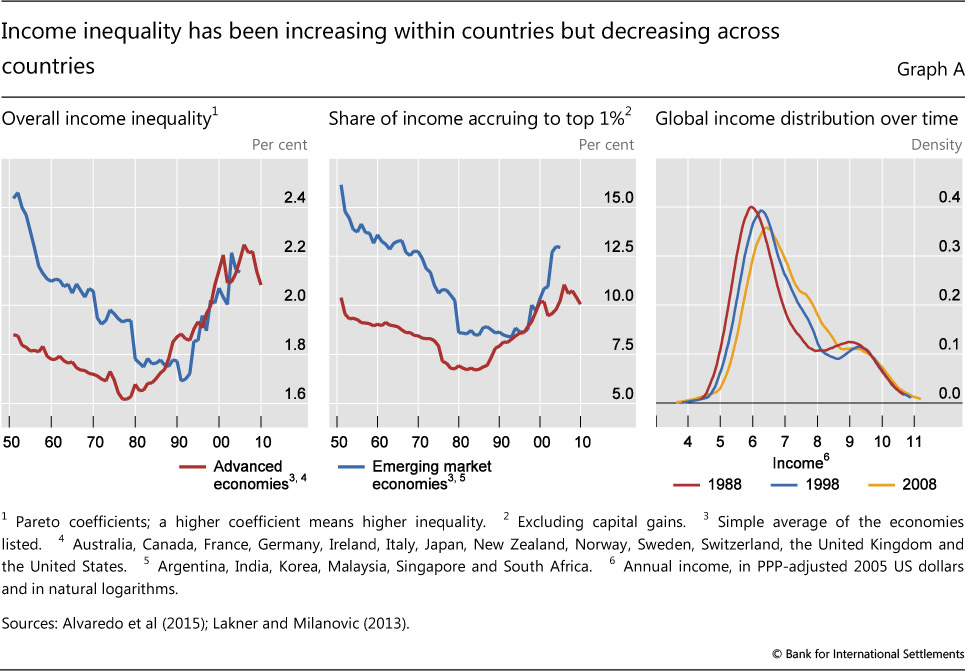
Within countries, income inequality has risen globally. Graph A (left-hand panel) shows that there is a U-shaped time pattern in average income inequality, a pattern that is observable across economies. After thinning in the 1950s, 1960s and 1970s, the right tail of the income distribution has been getting fatter. ; The same U-shaped pattern is found in the share of income accruing to the top 1% of the distribution (Graph A, centre panel), suggesting that the top end of the distribution is an important driver of inequality. Rising income inequality within countries contrasts with narrower income dispersion across countries. Between 1988 and 2008, the global income distribution narrowed: the bottom tail of the distribution shifted to the right (Graph A, right-hand panel).
 This shift largely reflects growth in middle-income EMEs, especially China.
Rising income inequality within economies and a lower dispersion of incomes across countries are consistent with global factors driving inequality trends. Economic and financial globalisation is thought to have widened the income distribution by increasing the ratio of skilled to unskilled wages. Highly skilled workers benefit from global opportunities, whereas the low-skilled face stiff competition from (cheaper) foreign labour and a loss of bargaining power. By the same token, workers in EMEs have seen their wages rise relative to those of their AE counterparts even as low-skilled wages have fallen relative to those of more skilled workers within AEs. This process has likely been supported by skill-biased technological progress and by advances in information technology in particular.
The integration of the labour force of large EMEs into global production has probably reduced the rate of return on labour relative to capital. As a consequence, the returns to wealth (ie corporate profits, dividends, rents, sales of property, capital gains) and the share of capital in total income have increased. Given that the distribution of wealth is more concentrated than the distribution of income, a rising capital share increases income inequality.
Moreover, the faster rise in remuneration at the very top of the income distribution relative to wage growth in the lower percentiles has been linked both to the rapid growth of the financial sector since the 1980s and to changes in the social norms that contribute to the determination of executive pay (Piketty (2014)).
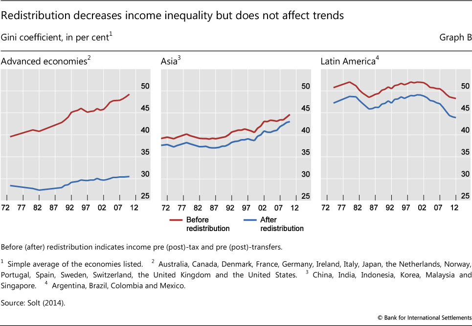
Redistributive fiscal policies appear have reduced the level of inequality, especially in AEs, but they have not changed long-term trends (Graph B).
The left-hand panel of Graph A plots time series of the Pareto coefficient - a measure that captures the higher-income part of the distribution. The higher the Pareto coefficient, the fatter the upper tail of the income distribution. For concreteness, if the Pareto coefficient is 2, the average income of individuals with income above $100,000 is $200,000 and the average income of individuals with income above $1 million is $2 million. Lakner and Milanović (2013) estimate the global distribution of income by aggregating within country household surveys. They correct for income underreporting at the top by using the discrepancy between consumption growth in national accounts and in household surveys. This is allocated to the top 10% of the income distribution by fitting a Pareto distribution to the upper tail. In the United States, for example, in 2010 the top 1% of households held about 35% of total wealth (see Graph 1, right-most panel) but 18% of total income (see Graph A, centre panel).
How has wealth inequality evolved since the crisis? To answer this question, this section simulates the impact of observed changes in asset values on the wealth of different quintiles of household wealth distribution in six AEs. We emphasise the direct effects of valuation changes on wealth inequality, preparing the ground for a discussion of the possible role of unconventional monetary policy.
Methodology
The simulation focuses on the impact of changes in interest rates and asset prices on wealth inequality, abstracting from active portfolio shifts by households. The main reason for this approach is the lack of comparable time series data on the composition of households' balance sheets. We use microdata from the household surveys of six AEs (France, Germany, Italy, Spain, the United Kingdom and the United States). Those surveys are heterogeneous: they are conducted at different times; are of low frequency (every two to three years); differ in the granularity of their coverage of assets and liabilities; and, in some cases, have only one observation.
In order to be able to compare the evolution of household wealth across countries, we use a single point-in-time observation on the composition of balance sheets based on a consistent definition of asset classes. By doing so, we are implicitly assuming that portfolio composition is independent of macroeconomic and financial conditions.3 This assumption can be justified by thinking of our simulation as a partial equilibrium exercise seeking to determine the impact of changes in asset prices and interest rates on wealth inequality while holding the composition of assets and liabilities constant.4
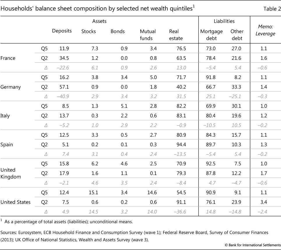
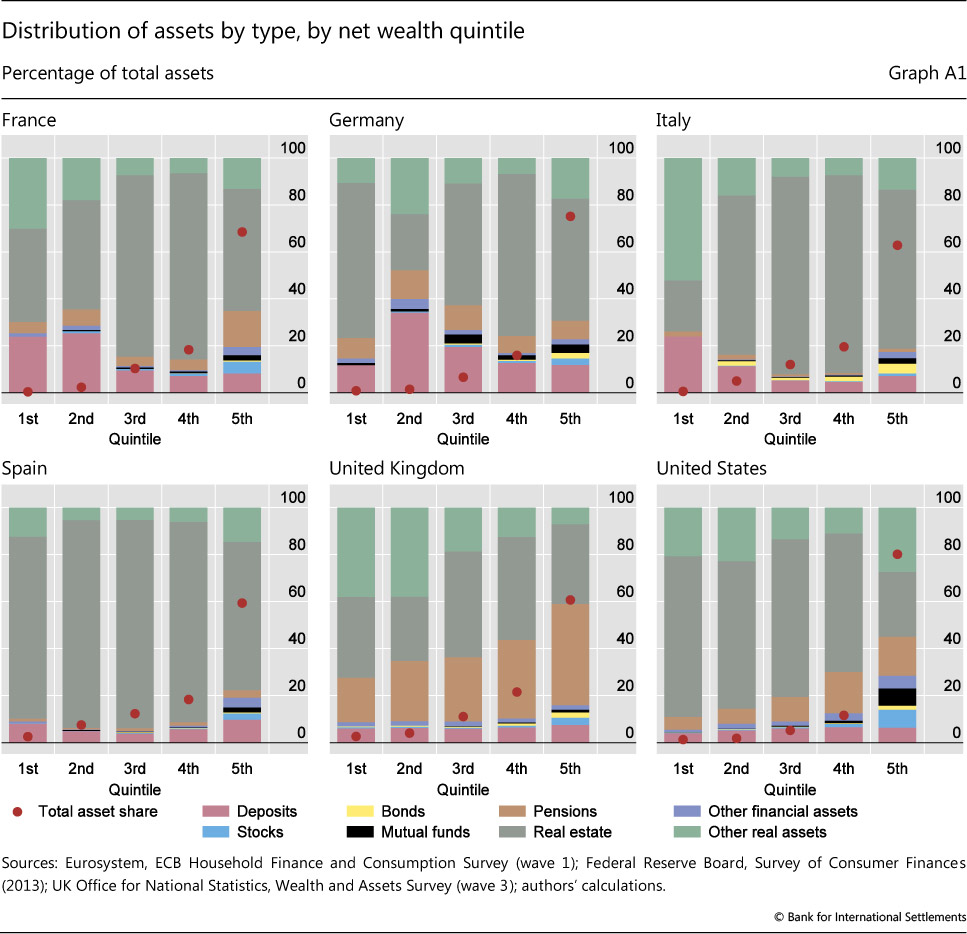
We proceed in three steps. As a first step, we use the survey data to construct household balance sheets for the first to fifth quintiles of the wealth distribution in each country. We thus obtain portfolio weights for a number of broad asset classes (deposits, bonds, stocks, mutual funds and housing) and liabilities (mortgage and non-mortgage credit).5 Balance sheets for the selected quintiles are reported in Table 2, and a more detailed breakdown is illustrated in Graph A1 in the Annex.
To construct comparable classes of assets and liabilities, we use categories reported in the ECB's Household Finance and Consumption Survey (HFCS). The first wave of this survey, which covers more than half of the countries in our sample, was released in 2013. For cross-country comparability, we chose survey years for the United Kingdom (WAS) and the United States (SCF) that would be as close as possible to those of the HFCS.6
The second step is to compute the growth rate of assets and liabilities. We assume that assets grow because of changes in asset prices and because cash flows are reinvested in the portfolio. Equivalently, there is no asset accumulation beyond cash flows, and no decumulation. As a result, the growth rate of assets is equal to the return on assets. For the sake of symmetry between the treatment of assets and liabilities, we assume that households do not pay down debt. Households issue only one-period debt and roll over both principal and interest in every period.7 Under these assumptions, the growth rate of liabilities is simply the cost of debt.
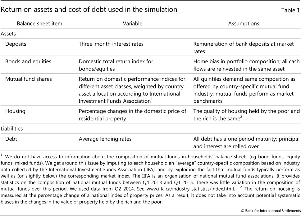
Since we have taken the composition of assets and liabilities to be fixed over time, the returns on assets and the cost of debt are simply linear combinations of the returns on the underlying assets and the cost of the underlying debt liabilities, weighted by their respective shares in total assets and liabilities (see Box 2). We use market data to determine asset returns and average lending rates to proxy for the cost of debt (Table 1). The resulting rates of return on assets and cost of debt liabilities are reported in rows 1 and 4 of Graph 2.
As a third and final step, we calculate our measure of wealth inequality as the ratio of the fifth quintile of the wealth distribution (q5) to the second quintile (q2), by analogy with percentile ratio measures commonly used for income inequality.8 By this metric, inequality increases when q5 accumulates wealth faster than q2 or, in other words, when the wealth growth differential between q5 and q2 is positive (see Box 2).9
Results
The composition of household balance sheets in AEs varies considerably between the lower and the upper ends of the wealth distribution. Table 2 shows the composition of assets and liabilities for selected quintiles of the net wealth distribution according to national surveys (Graph A1 in the Annex provides a more detailed breakdown). Asset portfolios at the top of the wealth distribution are relatively diversified, including in particular significant holdings of equities and bonds. This contrasts with rather concentrated household portfolios at the bottom. These consist primarily of real estate, and contain financial assets mainly in the form of deposits. Leverage generally declines as households become richer, reflecting the fact that "poorer" households borrow to finance assets such as residential property and durable consumer goods.
Considering the tails of the wealth distribution - not shown here - generally reinforces this picture. The share of securities holdings, equity in particular, tends to be even higher at the top 5% or 1% of the distribution. Conversely, housing accounts for a higher share in the lowest net wealth quintile, for which low net wealth is in many cases a reflection of high levels of mortgage debt. In a number of cases, net wealth is negative, suggesting that liabilities, in the form of mortgage, consumer and other debt, exceed assets.10
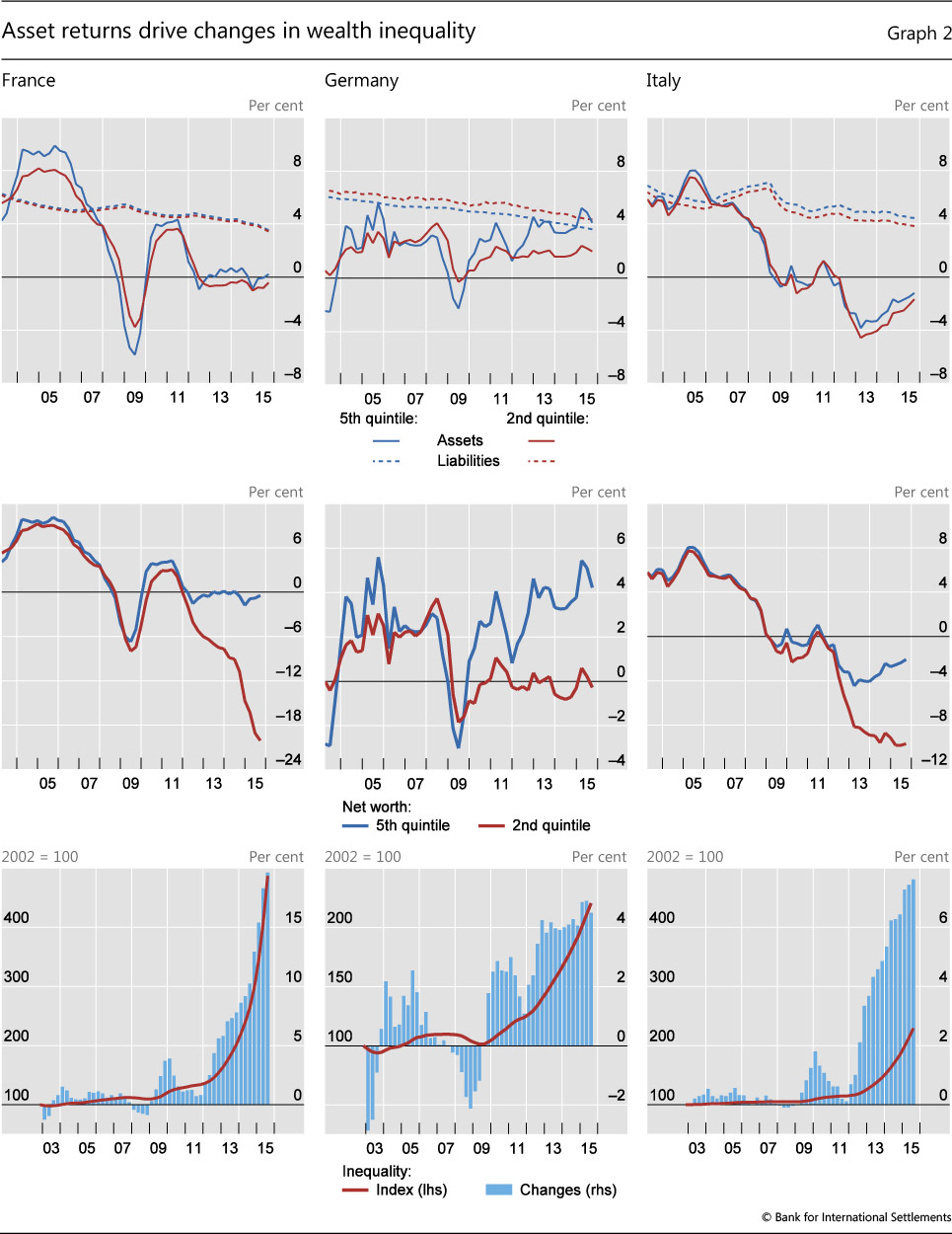
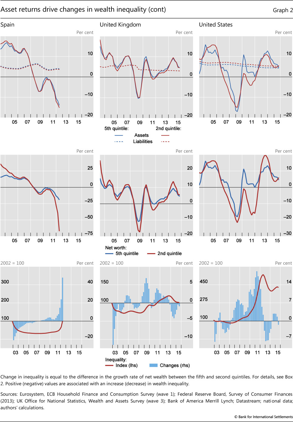
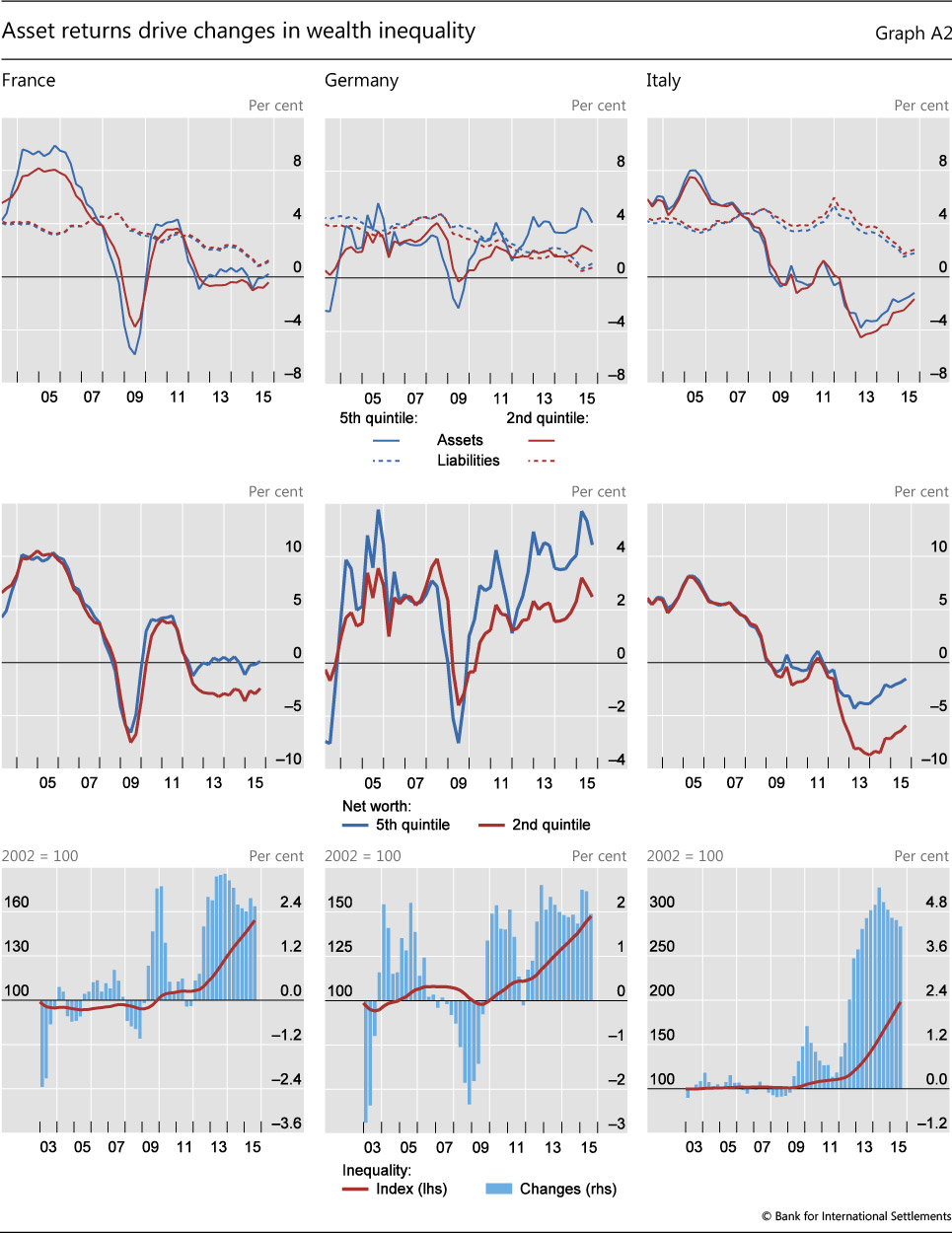
Results of the simulation of the evolution of wealth inequality are reported in Graphs 2 and 3. Graph 2 displays the time series of the returns on assets and the cost of liabilities (rows 1 and 4), wealth growth (rows 2 and 5) and the resulting quarterly changes in our measure of inequality together with the corresponding time series (rows 3 and 6).11 Graph 3 decomposes the difference between the return on assets of q5 and q2 by asset category, indicating which asset class has driven the changes.
Four main observations stand out. First, wealth inequality - measured as the ratio of the net wealth of "richer" to "poorer" households - has increased in most countries since the GFC. Bearing in mind the limitations of our simulation, the numerical results should be interpreted as a broad indication of trends, rather than precise orders of magnitude.
The blue bars in rows 3 and 6 of Graph 2 show quarterly changes in inequality.12 Drawing out a time series of cumulative changes in inequality by compounding these quarterly changes suggests that the crisis coincided with large increases in inequality (Graph 2, rows 3 and 6, red line). During the period covered by our simulation, the net wealth of richer households grew twice as fast as that of poorer ones in Germany and Italy, four times as fast in the United States and five times as fast in France. In the United Kingdom, inequality is back to its pre-crisis level after an initial decline.
Second, on the asset side, equity and housing have been the most important drivers of inequality (Graph 3). Although differences in the shares of equity holdings are typically small (below 7 percentage points in most countries except in the United States with around 25 percentage points; see Table 2), stocks have experienced consistently larger gains and suffered consistently larger losses than other asset classes. Since 2010, high equity returns have been the main driver of faster growth of net wealth at the top of the distribution.
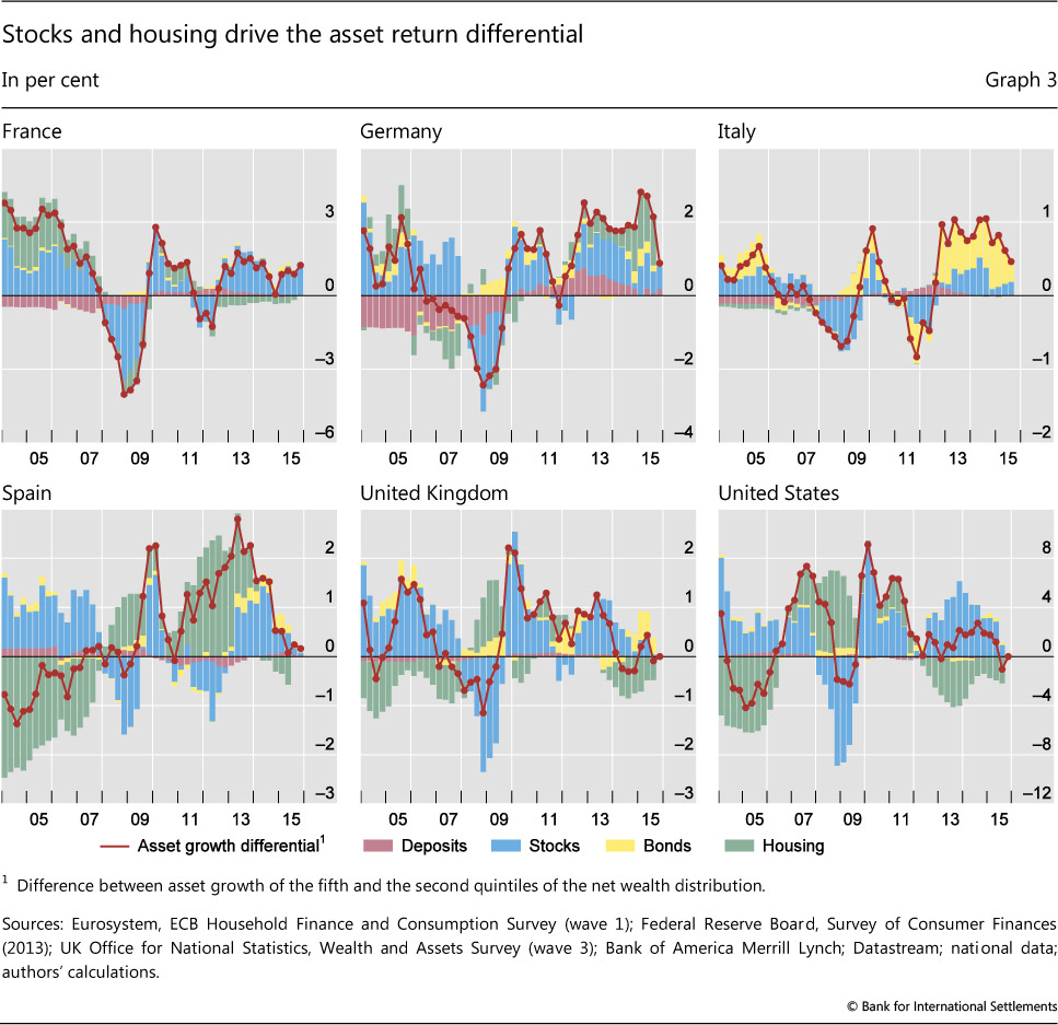
As regards housing, the combination of large swings in house prices and major differences in portfolio shares contributed significantly to changes in inequality. Over the past few years, the recovery of housing markets has tended to reduce wealth inequality in most countries, partly reversing the rise in inequality caused by the bust of housing markets during the GFC. Overall, the impact of equity prices on inequality seems to be much more cyclical, and less persistent, than that of house prices, which exhibit long booms and busts.
Third, fixed income assets - bonds and deposits - seem to have affected wealth inequality only in the trough of the recession between 2009 and 2010, and then again since 2012.13 One notable exception is Germany, where declining interest rates on deposits, which account for more than half of the assets of households in the lowest wealth quintile, have added to inequality. Our simulation may, however, overestimate the impact of lower interest rates in Germany: as in other countries, retail deposits are typically remunerated at rates that are stickier and lower than wholesale market rates. As a result, the change is likely to have been smaller than the one measured by our proxy.
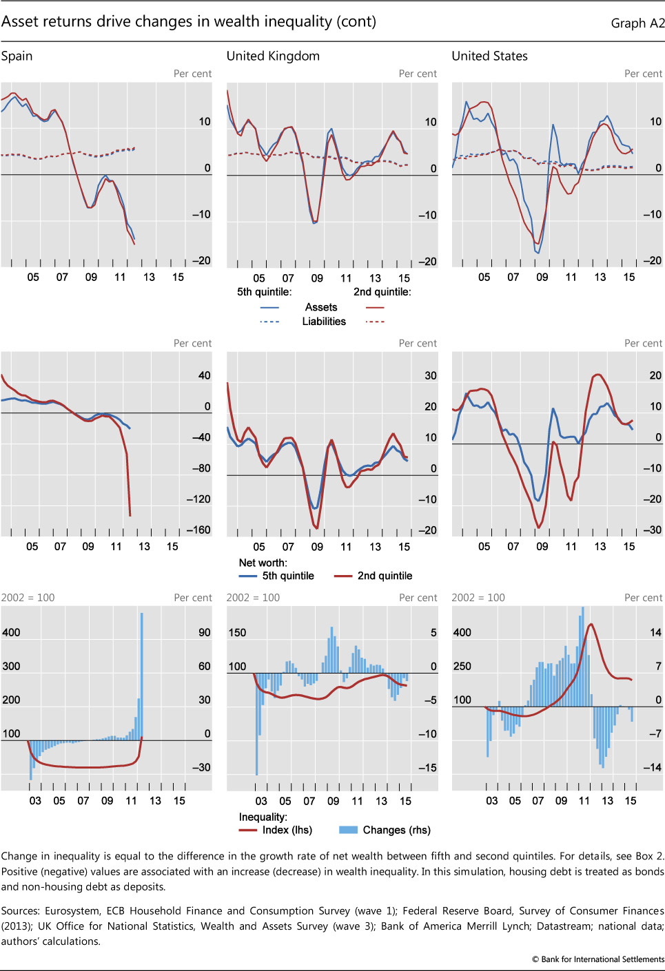
Finally, differences in household leverage have amplified distributional effects. Intuitively, when households are highly leveraged, asset gains (losses) have a larger impact on their wealth (see Box 2). The large wealth growth differential of Spanish households in q2 and q5 after 2010 is due to higher q2 leverage, as is the one experienced by US households between 2009 and 2013 (Graph 2, centre rows). In our simulation, these differentials accumulate over time to generate the large increases in inequality we observe in the sample (rows 3 and 6 of Graph 2, red line).14
Monetary policy as a possible driver of wealth inequality
Monetary policy may affect household wealth through different channels. Interest rate changes directly affect the valuation of both financial assets (eg equities and bonds) and real estate as well as the cost of leverage. Conventional easing of monetary policy by lowering short-term interest rates tends to boost asset prices. This works through a lowering of the discount rates applied to future income flows from these assets, and possibly by raising profit expectations and/or reducing risk premia.
At the same time, changes in financial conditions brought about by an easy monetary policy can either increase household savings and/or increase liabilities as households take on more debt. These channels tend to work with different time lags, further complicating the assessment of the overall effect.
Box 2
Some inequality arithmetic
Let a(q, t) and l(q, t) denote assets and liabilities of quintile q of the wealth distribution at time t, respectively. Defining a number A of asset classes and a number L of liability classes, we have that 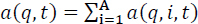 and that
 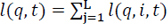 .
.
As discussed in more detail in the body of the text, we assume that the composition of household balance sheets at different quintiles of the wealth distribution is time-invariant. In practice, we fix the relative weights of different assets and liabilities on households' balance sheets. Let δ(q, i, t) = a(q, j, t) / a(q, t) denote the relative weight of asset i in the asset portfolio of quintile q at time t, with 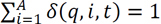 . Similarly, let δ(q, j, t) = l(q, j, t) / l(q, t) denote the relative weight of liability j in the liability portfolio of quintile q at time t, with
 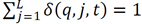 . Under the assumption of fixed weights,
  and
and  .
.
We use microdata from household surveys to construct the weights  and
and  . We consider five asset classes (A = 5) and two liability classes (L = 2). Under the assumption that there is no asset accumulation beyond capital gains and cash flows generated by each asset class (and no decumulation), the net growth rate of assets ∆a(q, t, t + 1) is simply a linear combination of the returns on assets,
  .
.
We use market data to construct quarterly time series of these returns,  . For liabilities, we assume that households issue one-period debt that is rolled over in every period. As a result, the quarterly time series of the net growth rate of liabilities ∆l(q, t, t + 1) is a linear combination of the underlying cost of debt,
  . The cost of mortgage and non-mortgage liabilities,
  , is built using average lending rates. Finally, to compute the time series of quintile leverage,
  , we combine survey data on the stocks of assets and liabilities at survey time τ, a(q, τ) and l(q, t), with the time series for asset returns and cost of liabilities. Applying the formula x(q, t + 1) = (1 +∆x(q, t, t + 1))x(q, t), for x = a, l allows us to recover time series for assets and liabilities. We then compute leverage as lev(q, t) = a(q, t) / (a(q, t) - l(q, t)). For all countries except Spain, our time series start in Q1 2003 and end in Q3 2015. For Spain, we end in Q2 2012, as in the most recent quarters "poor" households have negative wealth in the simulation (see also footnote 8).
Let w (q, t) denote the wealth of quintile q of the wealth distribution at time t, w (q, t) = a(q, t) − l(q, t). Our measure of wealth inequality is the ratio w (5, t) / w(2, t). Inequality increases over time if w(5, t + 1) / w(2, t + 1) − w(5, t) / w(2, t) >0, and decreases otherwise. Equivalently, inequality increases if the difference ∆w(5, t, t + 1) − ∆w(2, t, t + 1) > 0, where ∆x(q, t, t + 1) denotes the (net) growth rate of the variable x associated with quintile q between time t and time t + 1.
The growth rate of net wealth is given by the sum of the growth rate of assets and of liabilities, weighted by quintile leverage, ∆w(q, t, t +1) = ∆a(q, t, t + 1) lev(q, t) + ∆l(q, t, t + 1)(1 − lev (q, t)), with lev(q, t) = a(q, t) / w(q, t). As a result, the wealth growth differential between q5 and q2 is given by

Here, ∆w(q, t, t + 1) is the wealth growth rate of quintile q between quarter t and t + 1; ∆a(q, t, t + 1) represents the growth rate of assets, while ∆l(q, t, t + 1) denotes that of liabilities; finally, lev(q, t) is the leverage of quintile q in quarter t. Inequality increases if the left-hand side of equation (1) is positive, and decreases otherwise.
To tease out which underlying assets are responsible for the dynamics of the asset returns, we decompose the asset return differential as:

that is, as the sum of the "portfolio weight differentials", δ(5, i) − δ(2, i), weighted by the growth rate of the underlying asset, ∆a(i, t, t + 1). The decomposition in equation (2) is illustrated in Graph 3 in the main text.
All relevant quantities referred to in this box are nominal. We assign the values of assets and liabilities reported by the survey to the last quarter-year pair covered by survey-related fieldwork.
Notwithstanding the range of channels through which monetary policy may affect the distribution of wealth, the traditional view holds that such effects are small. As a by-product of the pursuit of macroeconomic stabilisation objectives, they net out over the business cycle. More generally, monetary policy that is neutral in the longer run should not have a lasting impact on inequality.
The role of unconventional monetary policies
Monetary policies in the aftermath of the GFC have raised questions about whether this assessment is still valid.
First, unconventional monetary policies have arguably relied more on wealth effects than conventional policy measures.15 With policy rates at, or even below, zero, central banks have directly aimed at influencing the composition of private sector portfolios and the price of risky assets. Portfolio rebalancing is thought to be one of the key channels for the transmission of unconventional policies (Bernanke (2012)). Communication about future policy intentions has also become more explicit (forward guidance) and has tried to steer market rates further out along the yield curve. In addition, by changing the size and composition of their balance sheets (balance sheet policies) central banks have begun to target financial conditions in specific markets (eg the housing market), and long-term interest rates and risk premia more generally.
Second, policy rates in major currency areas have been unusually low for an unusually long time - seven or eight years - which might suggest more persistent distributional effects than during a normal interest rate cycle. More fundamentally, this interest environment might be interpreted, in part, as the result of past policies that contributed to the financial busts which may give rise to questions about the long-run neutrality of monetary policy (Borio (2015)).
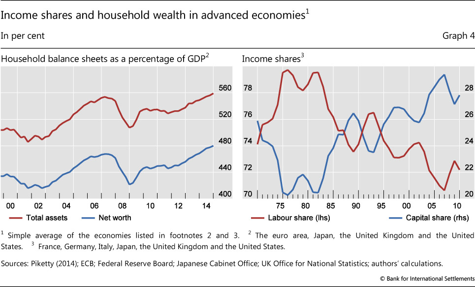
In addition, households may have become more sensitive to changes in interest rates and asset values over the past decade. For one, household balance sheets in AEs have expanded much faster than GDP, with total household assets and net wealth growing in tandem (Graph 4, left-hand panel). In addition, the share of capital income has been rising steadily since the 1980s and now accounts for about 30% of household income in AEs (right-hand panel).
Interpretation of the simulation results
While the simulation does not establish a direct link between wealth inequality and monetary policy, it sheds some light on the channels through which monetary policy might have had such effects. Four points stand out.
First, the simulation results suggest that the distributional effects of zero interest rates, forward guidance and large-scale asset purchases through their impact on bond prices have generally been modest. In particular, rising values of households' bond portfolios have not been associated with significant changes in wealth inequality. This is not surprising, given that the differences in the holdings of fixed income claims between "richer" and "poorer" households are generally relatively small.
Second, unconventional monetary policies might have had the most significant effects on the dynamics of wealth inequality through changes in equity returns and house prices.16 The evidence suggests that unconventional policies had a relatively strong and immediate effect on equity prices (see eg Rogers et al (2014)). As investors reshuffle their portfolios away from assets being purchased by the central bank towards other, potentially riskier, assets, the equity risk premium should decline, boosting equity prices further. And a low interest rate environment is likely to have encouraged a search for yield.
At the same time, lower interest rates should have supported real estate prices. House prices in the United States appear to have been positively affected by unconventional monetary policies (Gabriel and Lutz (2014)). The link between unconventional monetary policy and house prices has been relatively underexplored for the United Kingdom and the euro area. Nonetheless, it appears that central banks in these economies do pay attention to the possibility that unconventional measures may fuel housing booms.17
Third, for most countries in our sample, the net distributional effect of monetary policy depends on its relative impact on the value of housing assets and equities. Changes in house prices and equity returns tend to have opposite effects on inequality if housing assets are concentrated in "poorer" households and equity holdings are concentrated in "richer" ones.18 In these cases, to the extent that monetary policy has boosted equity prices more than house prices, it has tended to increase wealth inequality.
For illustration, consider the following example. In the United States, the share of equities in the portfolios of q5 households is about 15 percentage points higher than the corresponding share in the portfolios of q2 households while the share of real estate is about 35 percentage points lower. Hence, if monetary policy were to lift equity prices by 10%, it would have to raise house prices by about 4¼% to be distributionally neutral.
Finally, while monetary policy is likely to have contributed to lower borrowing costs, household leverage has further amplified the impact of lower asset returns on household inequality.
Conclusions
This feature has explored the recent evolution of household wealth inequality in AEs by simulating changes in the value of household assets and liabilities. The simulation results suggest that wealth inequality has generally risen in a sample of countries since the GFC.
The exercise provides tentative evidence of the relative importance of the channels through which monetary policy actions may have affected wealth inequality since the crisis. Taken at face value, our results suggest that the impact of low interest rates and rising bond prices on wealth inequality may have been small, while rising equity prices may have added to wealth inequality. A recovery of house prices appears to have only partly offset this effect.
However, important caveats apply when interpreting these results. First, the simulation is only a partial equilibrium exercise. Assets and liabilities vary over time not only because of valuation effects but also because of saving, borrowing and default, none of which are taken into account here. More fundamentally, our measure of wealth is incomplete. It does not capture the value of human capital, both in the form of the present value of future labour income and of accrued pension rights. As regards the former, monetary policy in the aftermath of the crisis obviously matters through its impact on unemployment and growth. Pension rights are not included in our study because of a number of conceptual challenges. That said, near zero or negative interest rates may well have had significant effects on such rights, not least through their impact on the viability of pension systems.
The empirical research on the nexus between monetary policy and inequality is still in its infancy. This reflects, on the one hand, the challenges associated with developing appropriate models that incorporate heterogeneous agents and the different channels through which monetary policy affects inequality. Moreover, data limitations are serious. This article suggests that further research on the distributional effects of monetary policy would be warranted. Because of their potential strength and persistence, understanding the distributional consequences of house price booms and busts - rather than the distributional impact of changes in bond prices - seems to be of particular importance.
References
Adam, K and P Tzamourani (2015): "Distributional consequences of asset price inflation in the euro area", University of Mannheim Department of Economics Working Papers, no 15.
Alvaredo, F, A Atkinson, T Piketty and E Saez (2015): "The World Top Incomes Database", topincomes.g-mond.parisschoolofeconomics.eu/22/01/2015.
Bernanke, B (2012): "Opening remarks: monetary policy since the onset of the crisis", proceedings of the Federal Reserve Bank of Kansas City Jackson Hole symposium, pp 1-22.
Borio, C (2015): "Revisiting three intellectual pillars of monetary policy received wisdom", speech at the Cato Institute, Washington DC, 12 November.
Cohan, W (2014): "How quantitative easing contributed to the nation's inequality problem", New York Times Deal Book, 24 October.
Draghi, M (2015): "The ECB's recent monetary policy measures: effectiveness and challenges", Michel Camdessus Central Banking Lecture, IMF, Washington DC, 14 May.
European Central Bank (2015): "The state of the house price cycle in the euro area", ECB Economic Bulletin, issue 6.
Frost, J and A Saiki (2014): "How does unconventional monetary policy affect inequality? Evidence from Japan", DNB Working Papers, no 423.
Gabriel, S and C Lutz (2014): "The impact of unconventional monetary policy on real estate markets", unpublished manuscript.
Giles, C (2014): "Data problems with Capital in the 21st century", Financial Times, 23 May.
Haldane, A (2014): "Unfair shares", remarks at the Bristol Festival of Ideas, 21 May.
Lakner, C and B Milanović (2013): "Global income distribution", World Bank Policy Research Working Papers, no 6719.
Mersch, Y (2014): "Monetary policy and economic inequality", keynote speech at the Corporate Credit Conference, Zurich, 17 October.
Piketty, T (2014): Capital in the 21st century, Harvard University Press.
Rogers, J, C Scotti and J Wright (2014): "Evaluating asset-market effects of unconventional monetary policy: a cross-country comparison", Board of Governors of the Federal Reserve System International Finance Discussion Papers, no 1101.
Saez, E and G Zucman (2014): "Wealth inequality in the United States since 1913: evidence from capitalised tax return data", NBER Working Papers, no 20625.
Solt, F (2014): "The standardized world income inequality database", SWIID Working Paper, version 5.0, October.
Wolf, M (2014): "Why inequality is such a drag on economies", Financial Times, 30 September.
Yellen, J (2015): "Economic mobility: research and ideas on strengthening families, communities, and the economy", speech at a community development research conference sponsored by the Federal Reserve System, Washington DC, 2 April.
Annex
1 The views expressed in this feature are those of the authors and do not necessarily reflect those of the BIS. We thank Claudio Borio, Ben Cohen, Mathias Drehmann and Hyun Shin for their comments. We also thank Sébastien Pérez-Duarte for his assistance with the Household Finance and Consumption Survey. Finally, we are grateful to Cristoph Lakner and Branko Milanović for sharing their estimates of the global distribution of income.
2 Serious data limitations render comparisons very difficult. There has been debate about the reliability of wealth estimates for the United Kingdom (Graph 1, third panel). The Financial Times took issue with Piketty's (2014) use of estate tax data from the UK authorities as those in charge of producing those data explicitly say that the data are best not used for the purpose of comparing wealth trends over time. The Financial Times (Giles (2014)) argued instead for using a survey of wealth in the United Kingdom; the latter data paint a different picture indicating that the share of wealth held by the top 1% of wealth holders in the United Kingdom is 44% rather than 71% (and has been flat in recent decades).
3 There is considerable cross-country variation in the frequency and availability of surveys. For instance, the ECB plans to release its Household Finance and Consumption Survey (HFCS) every three years (as is the case for the US Survey of Consumer Finances (SCF)) but currently only one wave exists (released in 2013). The UK Wealth and Assets Survey (WAS) is conducted on a biennial basis, starting in 2006.
4 Moreover, surveys that are available at several points in time suggest that portfolio composition has typically remained fairly stable.
5 An important asset class that we exclude from our simulation is pensions. One reason is a lack of comparability between countries with pay-as-you-go and funded pension schemes. Another is that even for funded schemes, methodological challenges loom large. Surveys record pension assets as the sum of the value of current occupational pension wealth, retained rights in occupational pensions, current personal pension wealth, retained rights in personal pensions, additional voluntary contributions, value of pensions expected from former spouses/partners and value of pensions in payment. It is important to emphasise that those are only estimates. Modelling is needed to calculate the value of current occupational pension wealth, retained rights in occupational pensions etc for each household. As a result, the estimates are not readily comparable across surveys. Moreover, computing the impact of valuation changes on pension assets is only a meaningful exercise if we think about current personal pension wealth and occupational pension wealth (ie claims on pension funds) for which the underlying composition is not reported in the surveys.
As illustrated in Graph A1 in the Annex, the importance of pension assets varies significantly across countries. For example, in countries where the social security component of the pension system is small (United Kingdom and United States), pension assets account for a relatively large share of total assets (38% and 16%, respectively). In euro area countries, by contrast, estimates of the share of pensions in total assets tends to be smaller (1.3% in Italy, 2.4% in Spain, 8% in Germany and 12% in France).
6 Survey fieldwork years: Germany: 2010-11; Spain: 2000-09; France: 2009-10; Italy: 2011; United Kingdom: 2011; United States: 2012.
7 In principle, we could also have compounded the changes in the market value of liabilities (ie the present discounted value of cash flows associated with the loans), which would have preserved symmetry. For this calculation, however, we would have needed detailed information on the maturity and type of loans, which is not available in the surveys.
As a way to test for the sensitivity of our results to different assumptions about the dynamics of liabilities, we repeat all calculations by allowing mortgage liabilities to compound at the same rate as that of bonds, and non-mortgage liabilities at the same rate as that of deposits, the idea being that liabilities should be treated as an asset with a negative sign (see Graph A2 in the Annex). A comparison of Graphs 2 and A2 reveals that the dynamics of inequality (as displayed by the red line in row 3 of the two graphs) are unchanged although for some countries there are considerable differences in the levels. For instance, when we allow liabilities to compound as bonds and deposits, inequality grows much less in France and in the United States.
8 We considered using the q5/q1 ratio. However, there are quarters in which q1 has negative wealth for some of the countries in our sample. In this case, the ratio is negative and it is no longer a meaningful measure of inequality. The q5/q2 ratio, on the other hand, is consistently positive with the exception of Spain after Q2 2012. In the latter quarters of the sample, the second quintile of the Spanish wealth distribution has negative wealth as assets decline at a faster rate than liabilities rise.
9 Combining the stocks of assets and liabilities at survey time with the growth rates computed in the second step, we can construct time series for both sides of the balance sheet. We can then compute leverage as the ratio of assets to assets net of liabilities.
10 These calculations do not take into account human wealth, that is, the capitalised value of labour income. As a result, they tend to understate the true value of household wealth.
11 The inequality time series are obtained by simple compounding based on quarterly changes.
12 For all countries in the sample, changes in wealth inequality are driven by the dynamics of asset growth. A comparison of rows 1 and 4, and 3 and 6, in Graph 2 indeed reveals that the wealth growth differential, ∆w(5, t, t + 1) − ∆w(2, t, t + 1), follows the same pattern as that of the asset return differential, ∆a(5, t, t + 1) − ∆a(2, t, t + 1).
13 This is consistent with the findings of Adam and Tzamourani (2015), who consider the distributional consequences of a 10% increase in bond, equity and house prices, respectively. Using HFCS data, they find that the impact of bond price changes on wealth inequality (as measured by percentage changes in the Gini coefficient) is negligible.
14 The wealth growth differential is highly sensitive to the way in which leverage is allowed to change endogenously in the simulation. As explained in Box 2, we combine the stocks of assets and liabilities at survey time with the time series for asset returns and the cost of debt to obtain time series for assets and liabilities, and a corresponding leverage series that matches the leverage ratio at survey time. If, instead, we had assumed a zero leverage differential between q2 and q5 at the beginning of the simulation, and allowed leverage to change endogenously with assets and liabilities (an approach that imposes no structure on leverage and allows it to be driven only by valuation changes in assets and liabilities), we would have obtained smaller leverage differentials throughout the simulation period, and therefore smaller wealth differentials.
15 The conventional view is that monetary policy works via intertemporal substitution effects and that the distributional effects that arise from changes in interest rates (say, between borrowers and savers) net out over the business cycle.
16 Frost and Saiki (2014) study the impact of unconventional monetary policy on income inequality in Japan in a vector autoregression (VAR) framework. Using household survey data, they find that quantitative easing widened income inequality, especially after 2008 when policy became more aggressive. They identify capital gains resulting from higher asset prices as the main driver.
17 Reporting on the state of the housing price cycle in the euro area, the ECB recently listed "non-standard monetary policy measures [-] designed to keep interest rates low for some time to come" as one of the factors supporting house prices (ECB (2015)).
18 In Italy, Spain, the United Kingdom and the United States, the "rich" hold relatively more stocks and the "poor" relatively more housing wealth. In other words, the "portfolio weight differential" between q5 and q2 is positive for stocks and negative for housing (see Table 2).