Volatility is back
Updated 21 March 2018: Graph A1 has been corrected.
Stock markets across the globe underwent a sharp correction in late January and early February. After a steady rally that had lasted several months, capped by the strongest January since the 1990s, the release of a labour market report showing higher than expected US wage growth heralded a burst of heightened activity. Equity valuations fell, rebounded and fell again, amid unusual levels of intraday volatility. This correction coincided with higher volatility in government bond markets. Long-term Treasury yields had been gradually rising since mid-December, as investors seemed increasingly concerned about inflation risks as well as the macroeconomic impact of US tax reform. A sudden spurt in yields at the very end of January preceded the stock market drop in the United States and subsequently in other advanced economies (AEs). Government bond yields also increased in several other AEs, as the synchronised upswing in global growth led investors to price in a less gradual than previously expected exit from unconventional policies.
Throughout the period under review, which started in late November, market participants remained very sensitive to any perceived changes in central banks' messages. As expected, the Federal Reserve raised the federal funds target range by 25 basis points in December, and its balance sheet reduction moved forward largely as planned. Across the Atlantic, the ECB maintained its policy stance and left its forward guidance unaltered, including an open-ended date for the termination of its asset purchase programme (APP). The Bank of Japan responded to an uptick in long-term yields, which appeared to test its yield curve control policy, with an offer to buy an unlimited amount of long-term government bonds.
The market tremors occurred within a general context of protracted US dollar weakness for most of the period, continued loosening of credit conditions, and undaunted risk-taking in most asset classes. A brief flight-to-safety event associated with the peak of the stock market turbulence provided only limited support for the dollar. Neither the Fed's steady tightening nor the recent equity sell-off coincided with wider corporate credit spreads, which remained at record lows. The appetite for emerging market economy (EME) assets also stayed strong. Stock markets soon stabilised and trimmed their losses. At the same time, bond investors appeared to struggle in assessing the overall impact of an evolving inflationary outlook and the uncertain size of the future net supply of securities with longer tenors.
Equity market correction triggered by inflation concerns
Equity prices rallied globally after the seasonal Christmas lull. During the first few weeks of January, the S&P 500 rose more than 6%, in one of the strongest starts to the year since the late 1990s. In those weeks, the Nikkei 225 jumped 4%, EME stock markets rose almost 10% and European stocks went up more than 3% (Graph 1, top left-hand panel). At the end of the month, the rosy picture changed abruptly. On 2 February, a stronger than expected US labour market report - stating that non-farm payrolls had risen 200,000 in January, while wages had increased 2.9% year on year - seemed to stoke market participants' concerns about a firming inflationary outlook. The payroll figures were above analysts' expectations, and were accompanied by news that job creation during 2017 had been revised upwards. But it was the large annualised increase in hourly earnings that received the most press coverage, being the highest rise in wages since the end of the recession in mid-2009. The figure was widely perceived as increasing the chances of a faster pace of monetary policy tightening by the Federal Reserve.
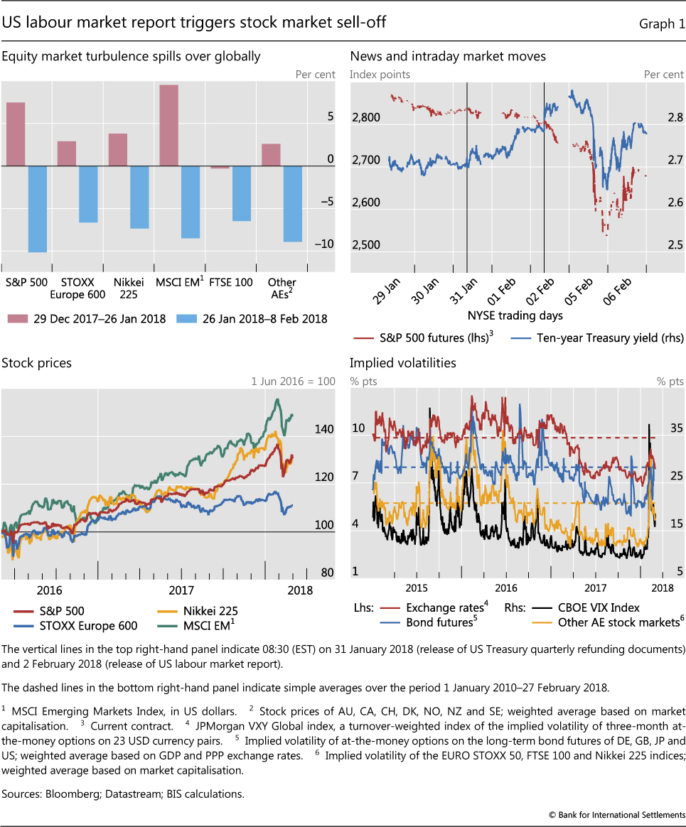
Global stock markets fell sharply in the wake of the report (Graph 1, top right-hand panel). During the week following its release, stock indices gave away the year's gains, and more, with the S&P 500 falling by further than 10%, the Nikkei by 7%, EME stock markets 8% and euro area stock markets 7% (top left-hand panel). There were indications that forced sales by commodity trading advisers and other momentum traders, in response to accumulated losses on their cross-asset positions, had helped amplify initial short-term market movements. Stock markets stabilised subsequently, and added moderate gains up to the end of February (bottom left-hand panel).
The declines in stock markets were accompanied - and possibly exacerbated - by a spike in volatility. Equity and exchange rate volatility - both realised and implied - had been falling for a while and had touched new all-time lows early in the new year (Graph 1, bottom right-hand panel). When the market indices started turning down, stock market implied volatilities skyrocketed, especially for the S&P 500, approaching levels last seen in August 2015, when markets were roiled by changes to China's foreign exchange policy. Implied volatilities in bond and foreign exchange markets jumped too, though staying within range of their post-Great Financial Crisis (GFC) averages. Volatility dynamics appear to have been accentuated intraday by trading patterns related to rapid adjustments in positions in complex financial products that had been used to bet on persistent low market volatility (Box A).
Bond yields rise, but financial conditions stay loose
A sharp increase in long-term US bond yields heralded the stock market stress. Bond yields, which had steadily increased by about 35 basis points from mid-December, rose sharply over the first two days of February. Prior to the surprising strength of the US labour market report on 2 February, which boosted 10-year yields by about 5 basis points, bond investors had already been rattled by the US Treasury's quarterly refunding plan, released on the morning of 31 January (Graph 1, top right-hand panel). The plan featured unexpected, albeit modest, increases in the auction size of all coupon-bearing nominal securities, including the benchmark 10- and 30-year bonds.
The rise in long-term yields steepened the US term structure, which had been flattening for most of last year. Short-term yields had been increasing from early September 2017, as the beginning of the Federal Reserve's balance sheet reduction process appeared imminent. The two-year yield rose by almost 100 basis points between September and the end of January, clearly surpassing the flat plateau that had prevailed during the first half of last year (Graph 2, left-hand panel). Meanwhile, long-term yields significantly trailed the shorter tenors, staying essentially flat until last December. The subsequent boost to longer yields coincided with the approval by the US Congress of a major tax reform package, which was seen as likely to spur a significant fiscal expansion (Graph 2, centre panel).
Box A
The equity market turbulence of 5 February - the role of exchange-traded volatility products
On Monday 5 February, the S&P 500 index fell 4% while the VIX - a measure of volatility implied by equity option prices - jumped 20 points. Historically, falls in equity prices tend to be associated with higher volatility and thus a rise in the VIX. But the increase in the VIX on that day significantly exceeded what would be expected based on the historical relationship (Graph A1, left-hand panel). In fact, it was the largest daily increase in the VIX since the 1987 stock market crash.
The VIX is an index of one-month implied volatility constructed from S&P 500 option prices across a range of strike prices. Market participants can use equity options or VIX futures to hedge their market positions, or to take risky exposures to volatility itself. Trading in both types of derivative instrument can affect the level of the VIX.
Because it is derived from option prices, theoretically the VIX is the sum of expected future volatility and the volatility risk premium. Model estimates indicate that the rise in the VIX on 5 February far exceeded the change in expectations about future volatility (Graph A1, centre panel). The magnitude of the risk premium (ie the model residual) suggests that the VIX spike was largely due to internal dynamics in equity options or VIX futures markets. Indeed, the considerable expansion in the VIX futures market - market size (ie total open interest) rose from a daily average of about 180,000 contracts in 2011 to 590,000 in 2017 - means such dynamics are likely to have had a growing impact on the level of the VIX.
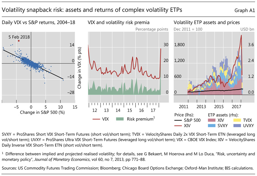
Among the growing users of VIX futures are issuers of volatility exchange-traded products (ETPs). These products allow investors to trade volatility for hedging or speculative purposes. Issuers of leveraged volatility ETPs take long positions in VIX futures to magnify returns relative to the VIX - for example, a 2X VIX ETP with $200 million in assets would double the daily gains or losses for its investors by using leverage to build a $400 million notional position in VIX futures. Inverse volatility ETPs take short positions in VIX futures so as to allow investors to bet on lower volatility. To maintain target exposure, issuers of leveraged and inverse ETPs rebalance portfolios on a daily basis by trading VIX-related derivatives, usually in the last hour of the trading day.
The assets of select leveraged and inverse volatility ETPs have expanded sharply over recent years, reaching about $4 billion at end-2017 (Graph A1, right-hand panel). Although marketed as short-term hedging products to investors, many market participants use these products to make long-term bets on volatility remaining low or becoming lower. Given the historical tendency of volatility increases to be rather sharp, such strategies can amount to "collecting pennies in front of a steamroller".
Even though the aggregate positions in these instruments are relatively small, systematic trading strategies of the issuers of leveraged and inverse volatility ETPs appear to have been a key factor behind the volatility spike that occurred on the afternoon of 5 February. Given the rise in the VIX earlier in the day, market participants could expect leveraged long volatility ETPs to rebalance their holdings by buying more VIX futures at the end of the day to maintain their target daily exposure (eg twice or three times their assets). They also knew that inverse volatility ETPs would have to buy VIX futures to cover the losses on their short position in VIX futures. So, both long and short volatility ETPs had to buy VIX futures. The rebalancing by both types of funds takes place right before 16:15, when they publish their daily net asset value. Hence, because the VIX had already been rising since the previous trading day, market participants knew that both types of ETP would be positioned on the same side of the VIX futures market right after New York equity market close. The scene was set.
There were signs that other market participants began bidding up VIX futures prices at around 15:30 in anticipation of the end-of-day rebalancing by volatility ETPs (Graph A2, left-hand panel). Due to the mechanical nature of the rebalancing, a higher VIX futures price necessitated even greater VIX futures purchases by the ETPs, creating a feedback loop. Transaction data show a spike in trading volume to 115,862 VIX futures contracts, or roughly one quarter of the entire market, and at highly inflated prices, within one minute at 16:08. The value of one of the inverse volatility ETPs, XIV, fell 84% and the product was subsequently terminated.
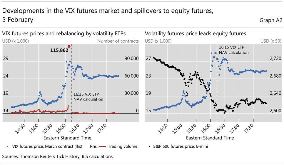
Spillovers back to the equity market on that day were also evident. For example, peaks and troughs in VIX futures prices led those of S&P (E-mini) futures (Graph A2, right-hand panel). One transmission channel worked via VIX futures dealers that hedged their exposure from selling VIX futures to the ETPs by shorting E-mini futures, thus putting further downward pressure on equity prices. In addition, normal algorithmic arbitrage strategies between ETFs, futures and cash markets kept the related market dynamics tightly linked. For the day as a whole, the S&P 500 index fell 4.2%, a 3.8 standard deviation daily move.
Overall, market developments on 5 February were another illustration of how synthetic leveraged structures can create and amplify market jumps, even if the core players themselves are relatively small. For investors, this was also a stark reminder of the outsize risks involved in speculative strategies using complex derivatives.
The four products shown include exchange-traded funds (ETFs), which give investors exposure to market risk, and exchange-traded notes (ETNs), which are debt securities backed by the credit of the issuers and expose investors to both market and credit risk. Neither the size nor the complex strategies of leveraged and inverse volatility ETPs are representative of the broader ETP market; see V Sushko and G Turner, "What risks do exchange-traded funds pose?", Bank of France, Financial Stability Review, forthcoming. As is common with debt securities, ETNs often come with an issuer call option to protect the issuer from losses. In the case of XIV, conditions of termination (called "acceleration" in the prospectus) include a loss of 80% or more from previous daily indicative closing value.
A firming inflationary outlook was at the root of the increase in US long-term yields during the period under review. US inflation stayed low in the backward-looking monthly figures, and survey-based measures of inflation expectations remained stable. But a stronger than expected CPI reading in mid-February highlighted market participants' nervousness about upward inflation risks, as the news was followed by yet another bout of yield increases and stock market softness.
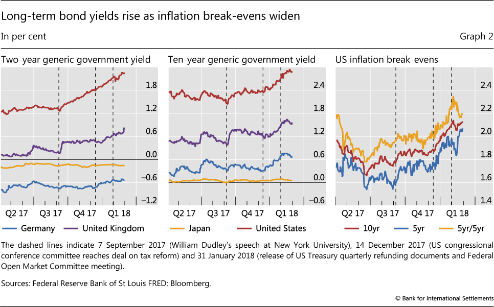
Market-based measures of inflation compensation have increased materially since mid-December. The 10-year break-even rate derived from US Treasury Inflation-Protected Securities (TIPS) crossed the 2% threshold soon after the turn of the year, and continued rising. Other gauges followed comparable paths (Graph 2, right-hand panel). The market-based inflation compensation measures decreased in the wake of the market turbulence. That drop was most likely related to the compression of nominal yields, as investors' flight to safety temporarily overwhelmed fixed income markets. Although the inflation break-evens rebounded as market volatility eased, by the end of February they were back around the levels immediately predating the turbulence.
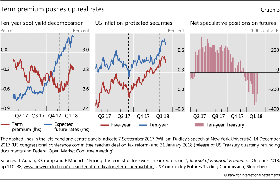
The expected path of future interest rates has also steepened substantially in recent months. In consonance with the gradual expected path of monetary policy tightening, the estimated expected future rate component of the 10-year zero coupon yield increased steadily from early September (Graph 3, left-hand panel). Similar developments across the maturity spectrum underlay increases in the shorter tenors of US Treasury securities.
The recent rise in long TIPS rates themselves (which should reflect real yields) may point towards the contribution of rising term premia to higher long-term nominal yields, in particular after the market turmoil. The 10-year TIPS yield had been slow to react to the Fed's balance sheet normalisation announcement in September, closing its spread over the five-year TIPS (Graph 3, centre panel). But after this spread stabilised in December, it rose again in the wake of the market moves of early February. This is consistent with the path followed by some estimates of the 10-year term premium. Such estimates must always be regarded with caution, as they may swing greatly depending on the features of the underlying model.1 Nevertheless, they suggest that while the term premium had been flat or declining from September to December, it started rising in January before jumping in early February (left-hand panel).
In other words, a sudden and persistent decompression of the term premium at the beginning of February, while inflation break-evens stabilised, pushed nominal and real yields higher. This suggests that inflation expectations largely drove yields until late January, with the term premium the driver of yields thereafter. The timing of the term premium decompression, following the release of the quarterly refunding plan, suggests that investors' reckoning of its implications for the future net supply of long-term securities may have played a role. In the short run, however, the large short position recently built by speculative investors may give way to additional volatility and occasional falls in long-term benchmarks in the event of "short squeezes" (Graph 3, right-hand panel).
Government bond yields also increased elsewhere, but mostly in the longer tenors. The synchronised strengthening of the global economy was seen as supportive of higher rates, especially at the long end, as investors seemed to anticipate a quicker exit from unconventional policies. Ten-year German bund yields rose to almost 0.80%, double the levels prevailing in mid-December (Graph 2, centre panel). Most of that increase occurred before the stock market turbulence, after which German long yields flattened. Short-term yields increased less (left-hand panel), with the result that the German term structure steepened over the period as a whole. The term structure remained roughly constant in Japan, where long yields barely moved at all, due in part to the forceful response of the Bank of Japan to upward pressure on yields in February.
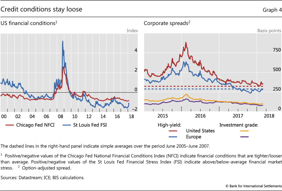
Despite equity market turbulence and higher yields, financial conditions remained very accommodative in the United States, with minimal signs of overall stress (Graph 4, left-hand panel). In fact, global credit markets were largely unfazed by these events. For instance, US and European corporate high-yield spreads had narrowed and stabilised after hitting their own bump in late November. When the turbulence struck in early February, they surrendered their January gains, but still ended up fluctuating around levels very close to their pre-GFC record lows (right-hand panel). Corporate investment grade spreads swung mildly, and eventually narrowed further.
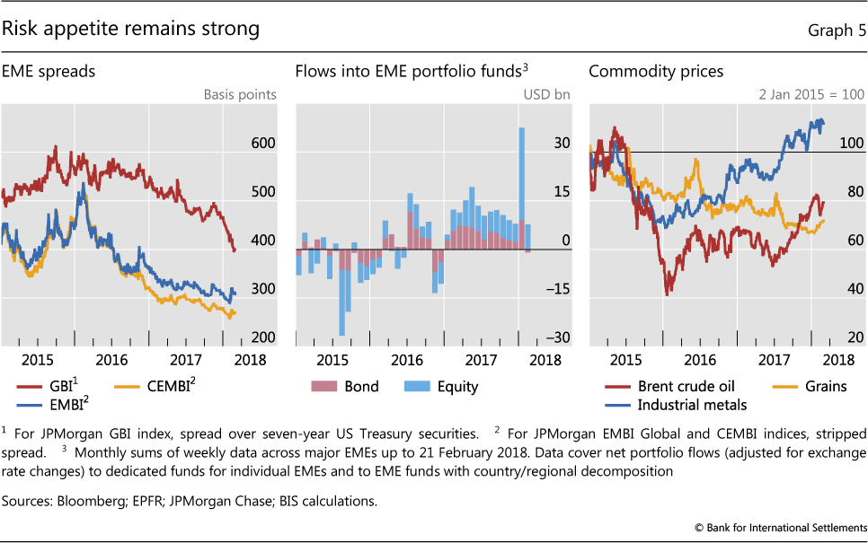
The financial outlook remained strong in emerging market economies as well. EME sovereign spreads compressed further, especially in the local currency segment: throughout the period, local currency spreads fell by 80 basis points on average vis-à-vis a decrease of 5 basis points in EMBI Global spreads (Graph 5, left-hand panel). Corporate EMBI spreads narrowed by about 10 basis points during the period under review. The strong performance of EME bond markets was underpinned by steady capital inflows, which reached a multi-year record high in January, after continued positive net inflows throughout 2017. Inflows to EME equity funds were more contained in February, whereas bond funds faced small redemptions (centre panel). There were no indications that appetite for EME debt and lending to other less established borrowers has waned. Finally, oil and other commodity prices saw some volatility during the equity market wobble, possibly because of de-risking by commodity trading advisers that exacerbated intraday movements. But all commodity indices ended with net gains by the end of the period (right-hand panel).2
Box B
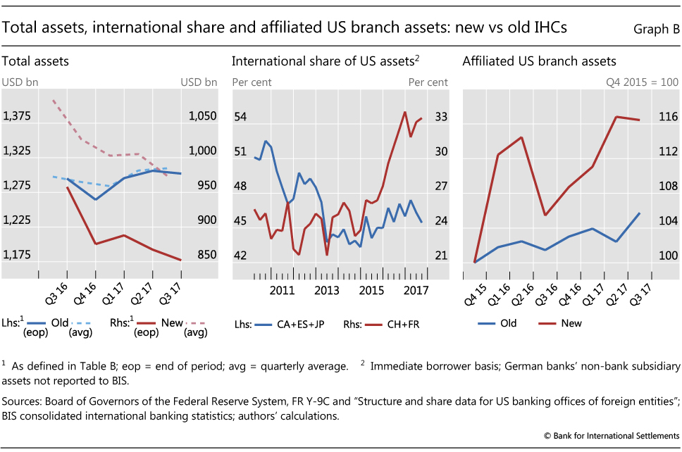
The new US intermediate holding companies: reducing or shifting assets?
Recent volatility in the US bond market recalls long-standing concerns about market-making capacity, especially for corporate bonds. This box examines how the balance sheets of foreign banking organisations (FBOs) with big US broker-dealers have responded to the implementation of the Dodd-Frank Act. Despite their reduction of assets subject to new US capital requirements, their market-making capacity in US corporate and agency bonds has not suffered.
This law required the Federal Reserve to enhance prudential standards for bank holding companies (BHCs) with assets over $50 billion, including through stress tests, capital plans and living wills. On the principle of "national treatment", the Fed required FBOs with $50 billion or more in US subsidiary (also known as "non-branch") assets to put all their US subsidiaries under an intermediate holding company (IHC) by 1 July 2016.
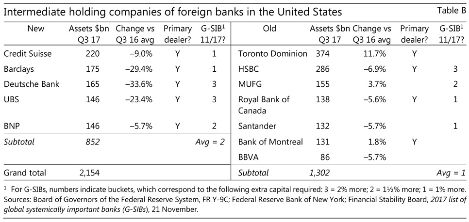
Foreign banks changed their operations and legal structures in response to this IHC requirement in several ways. Some squeezed subsidiaries' assets enough to avoid the IHC requirement altogether. Others already had separately capitalised BHCs, converted them into IHCs, and maintained or grew assets. Since these ("old") IHCs had largely adapted their operations to host capital requirements, we take them as a control group. Finally, five FBOs with Fed primary dealers, who had to set up new IHCs, have since reduced IHC assets (Table B) and appear to have also shifted assets to their offshore and US bank branches not subject to the US capital requirements.
Five banks on a 2014 Federal Reserve "illustrative list" of 17 banks that might have needed to set up IHCs ended up with subsidiary assets low enough not to do so. One of the five, Royal Bank of Scotland, had committed to its main owner, the UK Treasury, to downsize irrespective of the IHC threshold. Of the others, Société Générale had subsidiary assets over $50 billion as late as 30 June 2015 but managed them below the threshold by year-end.
Deutsche Bank established an IHC, but only after cutting its US subsidiary assets very substantially. Its former US BHC, named Taunus, had $355 billion in assets at end-2011 before it relinquished its BHC status in early 2012. Its new IHC reported assets at end-Q3 2016 of just $203 billion. Other FBOs may also have cut subsidiary assets before setting up new IHCs in 2016, again with the effect of limiting US capital charges, but data are lacking.
Since establishment, every new IHC has reduced its assets and therefore its required capital. Between Q3 2016 and Q3 2017, the new IHCs shrank their total assets by about $100 billion or 10% (Graph B, left-hand panel, either quarter-average or end-of-quarter). In contrast, FBOs with pre-existing BHCs ("old IHCs") kept their total US assets unchanged at $1.3 trillion. The new IHCs shrank their trading assets by $50 billion, moving or cutting Treasury securities but keeping agency and corporate bonds roughly unchanged. Trading asset levels at the old IHCs were stable.
If the new IHCs have shed assets in their US subsidiaries, did they also shift assets offshore? FBOs could do so either by rebooking existing assets or by booking new assets offshore. BIS consolidated international banking data are consistent with such a shift. In particular, Swiss and French banks have indeed grown (mostly offshore) international claims on US residents faster than locally booked claims on US residents (Graph B, centre panel). From a pre-IHC trough of 24% in 2014, the ratio of international claims on US residents of banks headquartered in these new IHC countries to their total US claims increased to 33% in the third quarter of 2017, an increase of 9 percentage points at the margin and a share increase of more than a third. In contrast, the ratio for the countries with banks operating with old IHCs barely increased, from 43% to 45%.
The FBOs with the new IHCs look to have shifted assets to US branches as well (Graph B, right-hand panel). From end-2015 to September 2017, US branch assets for FBOs with new IHCs increased by 16%. By contrast, during that same time, US branches of FBOs with old IHCs increased by 6%. If the branches affiliated with new IHCs had shown similar asset growth, their assets would have been $58 billion less. As with shifts of assets to foreign branches, operational, transfer accounting and legal constraints presumably limited the shifts from IHCs to their respective US branches.
We conclude that foreign banks facing the IHC requirement did not sit still. At least one FBO avoided the IHC mandate by shrinking assets while another cut assets significantly before the IHC deadline. All the new IHCs have subsequently reduced their footprints. Asset shifts within FBOs from IHCs to offshore or US bank branches would have reduced the specific US capital charges. One caveat is the limitation of our natural experiment: our control group with pre-existing BHCs has a greater weight of banking in their business models and, relatedly, a lower capital surcharge for consolidated size, interconnectedness, substitutability, span and complexity (Table B, "G-SIB?" column).
Any shrinkage of trading books by foreign-owned primary dealers could worsen the perceived disproportion between the huge stock of US corporate bonds outstanding and dealer inventory. Thus far, however, the new IHCs' asset reduction has spared their trading book of agency and corporate bonds.
Committee on the Global Financial System, "Fixed income market liquidity", CGFS Papers, no 55, January 2016. US Treasury, A financial system that creates economic opportunities: banks and credit unions, June 2017, suggests a higher threshold. "Factbox: Fed lists foreign banks that may fall under new rule", Reuters, 20 February 2014. Letters from the Board of Governors to Sheldon Goldfarb, General Counsel, RBS Americas, 11 December 2014, and to Slawomir Krupa, CEO, Société Générale Americas, 6 July 2016. Another of the five banks, Mizuho, expected to set up an IHC in the future according to the Board letter to Frank Carellini, Deputy General Manager, Mizuho Bank (USA), 18 February 2016. Deutsche Bank, Annual Report, 2011 and 2012, notes on subsidiaries; S Nasiripour and B Masters, "Bank regulators edge towards 'protectionism'", Financial Times, 12 December 2012.
Continued dollar weakness
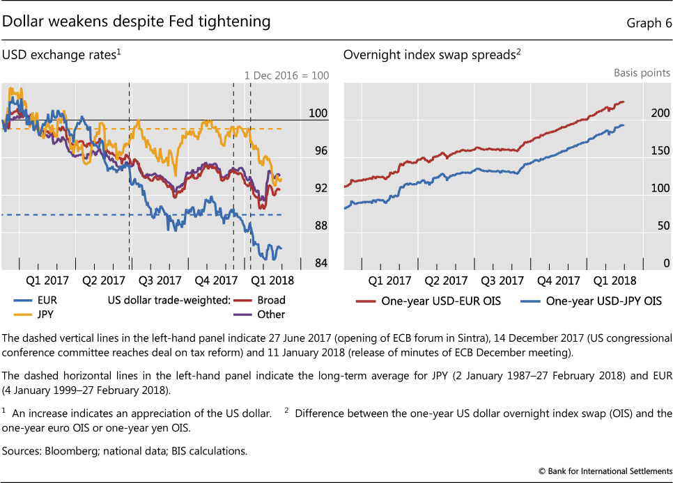
The stock and bond market developments took place against the broad backdrop of US dollar weakness. The dollar had been depreciating against most currencies since the beginning of 2017. The slide had been briefly arrested by last September's announcement of the start of the Federal Reserve's balance sheet run-off, but it resumed in December. The stock market correction interrupted it only briefly, in part because of the short-lived flight to safety that followed. By the end of February, the currency was down 1% from the beginning of the year, as measured by the broad trade-weighted index (Graph 6, left-hand panel).
The persistent weakness of the dollar is, in many respects, hard to reconcile with developments in monetary policy. Gradualism and predictability notwithstanding, the Federal Reserve has been steadily tightening its stance since December 2016. The central bank again raised the fed funds target range by 25 basis points in December 2017, and the future path of policy rates, as depicted by the "dot plot" of forecasts by members of the Federal Open Market Committee, stayed mostly unchanged. In contrast, the ECB did not set a termination date for its APP, and expected its key policy rates to remain unchanged long past the programme's horizon. The Bank of Japan signalled that qualitative and quantitative easing would continue. As a result, spreads between future expected short-term rates in the United States, on one side, and the euro area and Japan, on the other, continued to widen (Graph 6, right-hand panel).
That said, dollar weakness during a period of Fed policy tightening is not unusual. The dollar had also depreciated during the Federal Reserve's two previous tightening cycles in 1994 and 2004. In the course of the first 15 months of the current cycle, the dollar has depreciated by 11% against other AE currencies, as measured by the DXY dollar index. Over a similar time span, the dollar had depreciated by about 14% during the relatively stronger 1994 tightening, and by only 1% during the more gradual 2004 episode (Graph 7, left-hand panel), in each case as indicated by changes in the DXY index. However, the dollar had indeed appreciated, albeit moderately (3%), during the comparable window of the 1979 tightening. Both in 1979 and 1994, the bulk of the dollar appreciation occurred after the tightening cycle had finished.
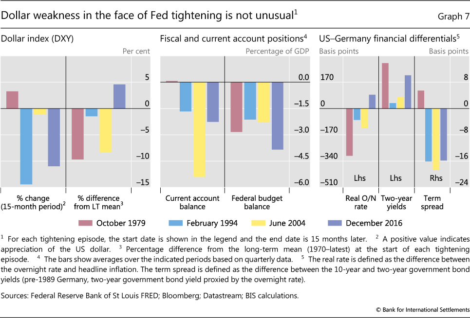
The position of the dollar at the beginning of the tightening vis-à-vis its long-term average value does not explain these exchange rate moves. Market commentary has emphasised that the relatively strong initial position of the dollar at the beginning of the current tightening cycle was a factor explaining its subsequent weakness. And in fact, in December 2016 the dollar was almost 5% above the average value of its index, computed for the full sample (Graph 7, left-hand panel). But the finding does not carry over to the other events. Both in 2004 (when the depreciation was small) and in 1979 (when the appreciation was moderate), the currency had entered the policy tightening episode 8-10% below its long-term average. In contrast, a dollar that was slightly below its mean in 1994 went on to depreciate almost 15% in the following months.
Similarly, market observers' emphasis on the role of the "twin deficits" (fiscal and external) is not clearly borne out by the data. True, the current account was slightly positive in 1979 (when the dollar appreciated) and negative in the other three events (when the dollar depreciated). But the external deficit in 2004 was more than double the one observed during 1994 and 2016 (Graph 7, centre panel), and yet the dollar depreciated much less in 2004. On the fiscal side, the average deficit-to-GDP ratio was roughly similar in the first three episodes, and higher in the current one. But fiscal consolidation was actually on the march in 1994, when the dollar depreciated most, while fiscal deficits were expected to increase during the other episodes because of significant tax cuts.3 While it is hard to find a clear link between the external deficits and the exchange rate in the data, protectionist rhetoric in the United States may have indeed played a role in the dollar's recent weakness, as well as statements by high-ranking officials that were understood to be aimed towards "talking down the currency".
Term spread differentials did exhibit patterns consistent with the exchange rate moves observed in these four incidents. Empirical research has shown that the term spread differential between two countries helps to forecast their currencies' exchange rate moves. The right-hand panel of Graph 7 suggests a simple "stylised fact": the dollar has depreciated whenever the term spread differential on average favoured other currencies, in this example Germany's. In other words, when the term spread tended to be higher in Germany than in the United States (even if the rates themselves were lower), the dollar depreciated, and vice versa. A causal explanation is not warranted, but the sign of the carry is likely to have played a role in supporting the appreciating currency. Other financial spreads typically examined by the exchange rate literature did not show consistent patterns across these four tightening episodes.
The dollar's depreciation has not been uniform across all currencies. In particular, the euro has proved especially strong. Since December 2016, the euro has appreciated by about 14% against the dollar. In contrast, during the same time span the yen has appreciated by 6% and other currencies by just under 6%. As the euro area economy continued to strengthen throughout last year, investors were increasingly pricing in a sooner than previously expected end to unconventional monetary policies, adding support for the currency. The ECB forum in Sintra in late June 2017 appeared to mark one of the main turning points (Graph 6, left-hand panel). The euro had been moving roughly in tandem with the yen and other currencies till then. Afterwards, it separated from the others, strengthening markedly and quickly converging towards its long-term average parity with the dollar, before the latter started depreciating further last December. The dollar's slide since December has appeared relatively broad-based; even the yen, which until then had been trading within a 5% range below its December 2016 level, also strengthened to stand well above its 30-year average parity.
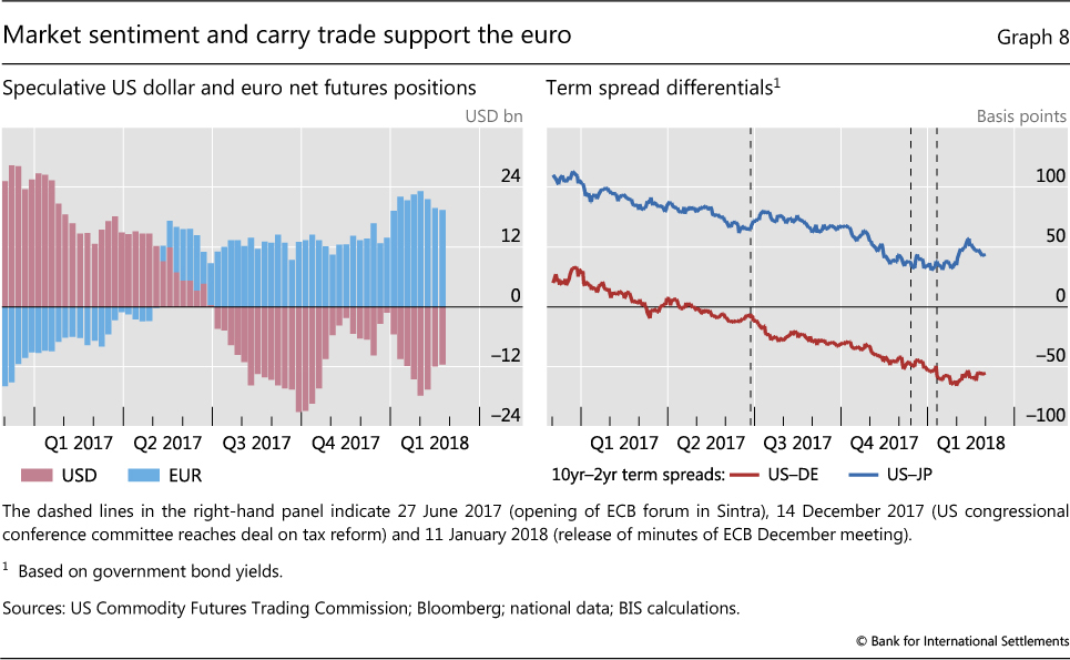
Market positioning and carry trades, at least in the short run, have been helping the euro. Investors' longstanding speculative net short euro position has been falling continuously since late 2016, and it turned into a net long position as of last June. Long euro positions spiked once again late last year (Graph 8, left-hand panel). Exactly the opposite happened on the dollar side. Moreover, as the term structure of US Treasuries flattened while that of German bunds gradually steepened, the term spread in Germany became consistently higher than the US term spread for the first time since the GFC (Graph 8, right-hand panel). The relative gap favouring German bonds and those of other core European economies reached almost 60 basis points in late February, despite some narrowing as turbulence took hold of markets.
1 The proper methodology and actual reliability of such estimates are a topic of discussion as well as the object of active research. Here, we rely on the daily estimates provided by the Federal Reserve Bank of New York, based on the methodology in T Adrian, R Crump and E Moench, "Pricing the term structure with linear regressions", Journal of Financial Economics, vol 110, no 1, October 2013, pp 110-38. This has become a common market barometer, as it is freely available at daily and monthly frequencies. See also BIS, "Term premia: concepts, models and estimates", 87th Annual Report, June 2017, pp 29-30.
2 Trading in credit and commodity markets was stable despite longstanding concerns that post-crisis regulations affecting market-making activity could reduce market resilience. Box B discusses how foreign banks in the United States, a number of which play an important role as market-makers, have responded to some of these new regulations.
3 This comparison should be interpreted with caution, as the timing of the various measures differed. In particular, the fiscal measures were adopted at different stages of the respective tightening cycles.