Securitisations: tranching concentrates uncertainty
Even when securitised assets are simple, transparent and of high quality, risk assessments will be uncertain. This will call for safeguards against potential undercapitalisation. Since the uncertainty concentrates mainly in securitisation tranches of intermediate seniority, the safeguards applied to these tranches should be substantial, proportionately much larger than those for the underlying pool of assets.1
JEL classification: G24, G32.
The past decade has witnessed the spectacular rise of the securitisation market, its dramatic fall and, recently, its timid revival. Much of this evolution reflected the changing fortunes of securitisations that were split into tranches of different seniority. Initially, such securitisations appealed strongly to investors searching for yield, as well as to banks seeking to reduce regulatory capital through the sale of judiciously selected tranches.2 Then, the financial crisis exposed widespread underestimation of tranche riskiness and illustrated that even sound risk assessments were not immune to substantial uncertainty.
The crisis sharpened policymakers' awareness that addressing the uncertainty in risk assessments is a precondition for a sustainable revival of the securitisation market. Admittedly, constructing simple and transparent asset pools would be a step towards reducing some of this uncertainty. That said, substantial uncertainty would remain and would concentrate in particular securitisation tranches. Despite the simplicity and transparency of the underlying assets, these tranches would not be simple.
We focus on the uncertainty inherent in estimating the risk parameters of a securitised pool and study how it translates into uncertainty about the distribution of losses across tranches of different seniority. The uncertainty could be small for junior tranches, which are the first to be wiped out following even small adverse shocks, or for tranches that are senior enough to enjoy substantial credit protection. In the middle of a securitisation's capital structure, however, mezzanine tranches would be subject to considerable uncertainty because of the so-called cliff effect: a small estimation error could mean that the risk of such a tranche is as low as that of a senior tranche or as high as that of a junior tranche.
Pool-wide uncertainty concentrates in tranches in the vicinity of the cliff and, if ignored, raises the possibility of severe undercapitalisation for these tranches. Based on a stylised example, our analysis reveals that this possibility is substantial even for extremely simple and transparent underlying assets. And while regulatory capital tends to increase with assets' riskiness, ignoring uncertainty results in a similarly elevated degree of undercapitalisation throughout. Safeguards are thus needed to address this issue head-on. Since the issue pertains mainly to mezzanine tranches, the safeguards applied to them should be proportionately much larger than those for the underlying asset pool. The revisions to the regulatory framework for securitisations - as proposed in a recent consultative document of the Basel Committee (BCBS (2013)) - are a welcome step in this direction.3
The article proceeds as follows. The first section reviews briefly the issuance and rating performance of securitisation tranches. Abstracting from uncertainty and adopting the benchmark credit risk model that underlies the Basel capital framework, the second and third sections compare capital requirements across different types of securitisation exposures. Finally, considering an extremely simple and transparent securitisation, the fourth section studies the potential undercapitalisation of tranches when model parameters are uncertain but treated as known, ie when no allowance is made for estimation error.
Historical experience with securitisation tranches
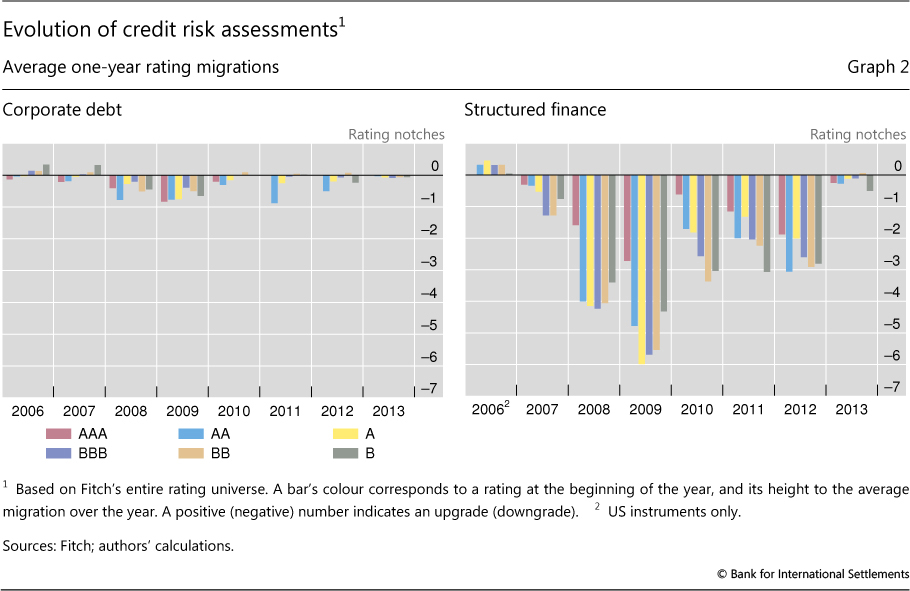
Extremely popular before the global financial crisis, structured securitisations underperformed subsequently. The issuance of such instruments grew strongly between 2003 and 2007 (Graph 1). As the crisis unfolded, however, outsize and widespread downgrades forced banks to quickly raise capital for unshed securitisation exposures.4 While the average rating of corporate bonds was revised downwards by roughly one notch in 2009, the corresponding revision was three to six notches for tranches with different seniority in securitisations' capital structure (Graph 2).5 And while the wave of downgrades quickly receded for corporate bonds, it persisted until 2012 for both low- and highly rated tranches.
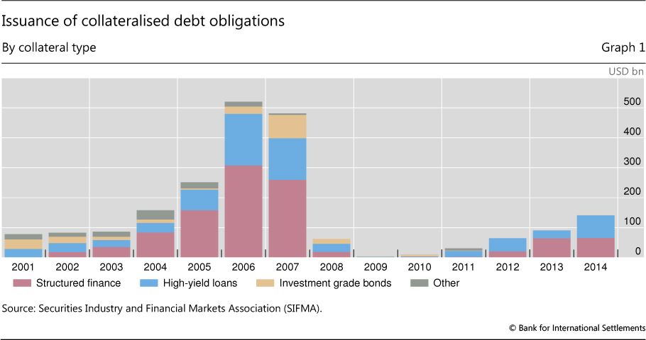
This relative rating performance underscored previously underappreciated features of structured securitisations and brought their issuance to a halt (Graph 1). Fender et al (2008) explained tranches' relative performance with the high sensitivity of their credit rating to changing economic conditions. In turn, the argument below points to an explanation of why tranche downgrades caught markets by surprise: market participants ignored substantial uncertainty in risk assessments.
Regulatory capital: from total portfolio to tranche exposures
A key function of capital is to protect against failure by absorbing losses. The internal ratings-based approach in the current regulatory capital framework for the banking book evaluates the probability distribution of portfolio credit losses on the basis of a stylised model. And it sets regulatory capital to a level that these losses could only exceed with a sufficiently small probability.
Assuming that the regulatory model is correct and its parameters are known with certainty, we outline in this section the calculation of capital at the level of the overall bank portfolio and the allocation of this capital to individual exposures. The ultimate goal of the section is to highlight the sensitivity of exposure-level regulatory capital to risk parameters. Awareness of this sensitivity - and how it differs across exposure types - leads us naturally to explore the implications of parameter uncertainty in the next section.
Regulatory capital for a credit portfolio
The regulatory model for portfolio credit risk is a stylised description of a bank's future losses. It aims to specify the average level of losses - which can be determined in advance - as well as possible deviations from the average. These unknown, random deviations are the credit risk against which the bank builds a capital cushion. The regulatory model's distinguishing feature - a single source of risk for the aggregate portfolio - stems from two assumptions.
The first assumption is that the portfolio comprises a very large number of small assets, ie the portfolio is asymptotic. When there are many assets, an adverse shock in one place - eg a personal tragedy of an uninsured homeowner - is sure to go hand in hand with a favourable shock elsewhere - eg a successful patent sale by an indebted enterprise. And when the assets are of comparably small size, such idiosyncratic shocks balance each other: asset-specific risks are diversified away at the portfolio level. If the portfolio were subject only to such idiosyncratic risk, actual losses would be known for sure, ie there would be losses but no credit risk at the level of the portfolio as a whole.
The second modelling assumption is that there is a single additional source of risk and it cannot be diversified away. This common risk factor is interpreted as relating to general economic conditions. For example, it may capture unexpected swings in energy prices or natural catastrophes that affect all assets in the portfolio. It thus generates correlation of losses and maintains portfolio credit risk.
The two assumptions are the reason why the regulatory model is referred to as the Asymptotic Single Risk Factor (ASRF) model. The parameters of this model - such as individual probabilities of default (PD), loss-given-default (LGD) and dependence on the common factor - shape the mapping from the common factor to portfolio losses. Provided that these parameters are known with certainty, the mapping is one-to-one: if the trajectory of the common factor were known, so would be aggregate portfolio losses.
The regulatory target is to limit the one-year likelihood of bank failure to 0.1%. This requires setting regulatory capital to a critical level of one-year portfolio losses that can be exceeded only with 0.1% probability. Under the ASRF model, these losses conveniently correspond to a critical level of the common factor: its 0.1 percentile. Thus, the bank's regulatory capital is equal to the portfolio losses that would materialise if the common factor were at its critical level (see Annex 1 for further details).
Exposure-level regulatory capital
In turn, the capital allocated to a particular exposure is equal to the exposure's contribution to the critical level of portfolio losses. Namely, it is equal to the expected losses on the exposure - roughly, the product of its PD and LGD - conditional on the common factor being at the chosen critical level (henceforth, "conditional expected losses"). This holds irrespective of the exposure type, eg a loan, a securitisation of loans or a securitisation tranche.
Even though exposure-level capital is always based on the same risk metric - conditional expected losses - its actual value would depend on the exposure type and the risk characteristics of the underlying assets. To focus on the importance of the exposure type, we keep risk characteristics as simple as possible. Namely, we focus on homogeneous loans - which have the same size and risk parameters - and on only one risk parameter - the unconditional PD - keeping LGD and common-factor dependence in the background at benchmark levels (see Annex 1). We treat these loans as underpinning exposures that are infinitesimally small parts of the bank's overall ASRF portfolio.
Exposures underpinned by a simple aggregation of homogeneous loans would face proportionately the same regulatory capital. For instance, if the PD of a loan is 3%,6 the capital allocated to this loan would be $0.10 per $1 of exposure. Pooling many such loans in a securitisation would then call for summing up the individual requirements, resulting again in regulatory capital of $0.10 per $1 of exposure.
Likewise, the same regulatory capital would apply to a composite exposure that consists of an equal fraction of each underlying loan, often referred to as a vertical tranche. An increase in the capital requirements for a loan would trivially translate one-to-one into an increase in the requirements for the pool of loans or for a vertical tranche from this pool. Across all these exposure types, the structure of the underlying risks does not change from the point of view of the metric used for regulatory capital, ie they all feature the same conditional expected losses per unit of exposure.
The picture changes dramatically when the securitisation is sliced into tranches of different seniority, which absorb pool losses sequentially. In this case, conditional expected losses are no longer distributed uniformly across tranches but are mostly concentrated in only some of them. And so is regulatory capital. We next show that the high concentration makes the regulatory capital for tranches of intermediate seniority substantially more sensitive to risk parameter values than the capital for a vertical tranche.
Regulatory capital for tranches of different seniority
Unlike vertical tranches, tranches that absorb losses sequentially offer a spectrum of risk characteristics and, thus, appeal to a broader investor base. Such tranches are defined by an attachment and a detachment point. The attachment point indicates the minimum of pool-level losses at which a given tranche begins to suffer losses. In turn, the detachment point corresponds to the amount of pool losses that completely wipe out the tranche.
The riskiness of a tranche decreases with the tranche's seniority in the securitisation's capital structure. A junior tranche, for example, could have attachment and detachment points equal to 0% and 10%, respectively, of the pool exposure. Such a tranche would be intact if there are no losses but would be partly eroded with the first losses. The erosion will be complete when losses reach 10% of the pool exposure. By contrast, a mezzanine tranche with attachment and detachment points of 10% and 20%, respectively, is initially protected but would be affected as soon as losses exceed 10% of the pool size. Finally, a senior tranche with attachment and detachment points of 20% and 100% respectively will be the most protected, starting to incur losses only when both the junior and mezzanine tranches are wiped out.
For given attachment and detachment points, the risk of a tranche would depend on the risk characteristics of the underlying pool. Our main focus is on the underlying assets' PD, which we first study in an ASRF pool. Besides this PD, however, the proposed revisions to the regulatory framework for securitisations take explicit account of several additional risk characteristics, such as the number of assets in the pool (ie the pool's granularity) and the correlation of associated losses (BCBS (2014), pp 10 and 31). In line with these proposals, we relax the ASRF assumptions at the level of the pool and study the robustness of our findings to the presence of idiosyncratic risk and to a second, pool-specific risk factor. In each case, we calculate "regulatory" capital as the expected loss on a tranche, conditional on the critical level of the global common factor.7
Perfectly diversified pool with a single common risk factor
We first study an ASRF pool, which possesses the two key properties of the bank's overall portfolio: full diversification of idiosyncratic risk and exposure to a single common risk factor. Paralleling the bank's portfolio, knowledge of the critical level of the common factor implies knowledge of the critical level of pool-wide losses. Given a loan PD of 3%, this level - and, thus, pool-wide capital - is equal to $0.10 per $1 of exposure.
Knowledge of the conditional pool losses translates into knowledge of the conditional losses on each tranche. By construction, a tranche with a detachment point below 10% of the pool size is sure to be fully wiped out when the common risk factor is at its critical level. Thus, the regulatory capital for such a tranche is $1 per $1 of exposure. By contrast, a tranche with an attachment point above 10% is fully shielded from losses when the common factor is at its critical level. The regulatory capital for this tranche is thus $0.
This story is depicted with the red line in Graph 3 (left-hand panel), which plots the dependence of regulatory capital on the seniority of a tranche from the ASRF pool. The height of this line shows the regulatory capital per unit of exposure to an infinitesimally thin tranche, whose attachment and detachment points coincide. As the pool's conditional losses are entirely concentrated in the most junior 10% of the tranches, so is the pool's capital. And the vertical segment of the red line at 0.1 illustrates the extreme version of the so-called cliff effect.
The cliff effect is less dramatic for a thick tranche (Graph 3, right-hand panel, red line). The regulatory capital for such a tranche, which has different attachment and detachment points, is equal to the aggregate capital for the thin tranches between these points. Aggregating across thin tranches on the two sides of the cliff dampens the effect of thick tranche seniority on regulatory capital (the red line is less steep in the right-hand than in the left-hand panel of Graph 3).
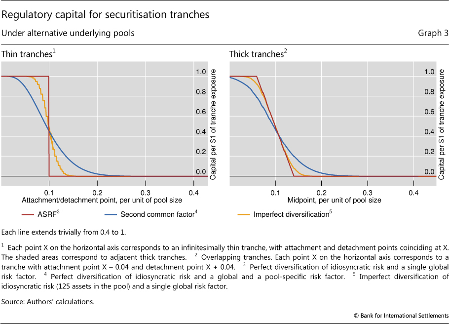
The cliff effect shapes the sensitivity of a tranche's regulatory capital to risk parameters. To see this, suppose that an increase in the PD of the underlying assets raises the ASRF pool's regulatory capital from $0.10 to $0.12 per $1 of exposure. Being subject to the extreme version of the cliff effect, a thin tranche with attachment/detachment points at 11% would see its regulatory capital rise by the maximum possible amount: from $0 to $1 per $1 of exposure. Given the less pronounced version of the cliff effect in the context of thick tranches, the corresponding rise for a 7%-15% tranche would be lower, albeit still substantial: from $0.38 to $0.63. By comparison, a vertical tranche, which is not subject to the cliff effect, would see its regulatory capital rise only as much as that for the overall pool: from $0.10 to $0.12 per $1 of exposure.
Imperfectly diversified pool or second common factor
The two assumptions that give rise to the extreme version of the cliff effect - full diversification of idiosyncratic risk and a single common risk factor - may be too strong. If either of these assumptions is violated within a securitised pool, knowledge of the global common factor would no longer imply knowledge of pool-wide losses. Conditional on the critical level of the global factor, there would be residual risk, which we study in the context of two different pools.
Illusory AAA tranches: the case of resecuritisations
Instead of comprising individual bonds or loans, the pool underlying a securitisation may itself comprise other securitisations or tranches of securitisations. For instance, the run-up to the global financial crisis witnessed the rise of securitisations of mezzanine tranches, or mezzanine resecuritisations. From 2005 to 2007, the senior tranches of mezzanine resecuritisations could rely on a wide investor base thanks to perceptions that they were virtually risk-free. Such perceptions turned out to be wrong. This box argues that the poor performance of senior tranches of mezzanine resecuritisations during the crisis can be explained with an overlooked inherent feature of these resecuritisations: high correlation of the underlying assets.
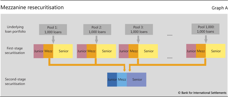
The box uses an illustrative example of a two-stage securitisation. In the first stage, 1 million homogeneous loans are split equally into 1,000 pools and then each pool is securitised. All first-stage securitisations are divided in the same way into junior, mezzanine and senior tranches. In the second stage, the 1,000 first-stage mezzanine tranches are all pooled together and securitised: this is a mezzanine resecuritisation (Graph A). The goal of the second-stage securitisation is to create a senior tranche that is subject to so little risk that it merits a AAA rating.
The risk characteristics of a first-stage mezzanine tranche would differ from those of an individual loan. Such a tranche is shielded by the corresponding junior tranche from the first losses on the underlying pool, ie from the losses triggered mainly by loan-specific, idiosyncratic shocks. Nevertheless, the mezzanine tranche is exposed to widespread, systematic shocks that are strong enough to completely wipe out the junior tranche. And the same systematic shocks would also dominate in mezzanine tranches from other first-stage securitisations. In turn, the greater relative role of systematic shocks in the mezzanine tranches than in the individual underlying loans implies that the losses on these tranches would be more strongly correlated than loan losses.
For a numerical illustration of this argument, let expression (A.1) in Annex 1 govern the credit risk of each securitised loan, and let the attachment and detachment points of each first-stage mezzanine tranche be equal to 3% and 7% of the respective pool. For a given homogeneous loan-level PD, the regulatory capital formula provides a common-factor loading that governs the correlation of defaults. Over a range of PDs from 0.3% to 2%, losses on first-stage mezzanine tranches are substantially more correlated than loan defaults. For any pair of loans, if there is at least one default, the likelihood of two defaults is lower than 3%. In the context of mezzanine tranches, the corresponding likelihood is 20 times larger. Namely, if at least one of two first-stage mezzanine tranches is subject to default losses, the other is as well with likelihood greater than 60%.
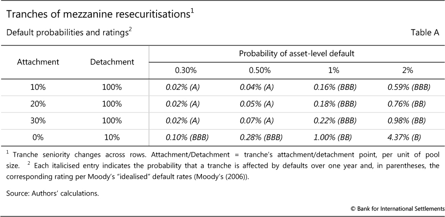
The strong correlation of losses on first-stage mezzanine tranches undermines the benefits of pooling these tranches together at the second securitisation stage. The higher this correlation, the smaller is the scope for diversification and the higher is the probability of large losses on the mezzanine resecuritisation. In fact, for the mezzanine resecuritisations implied by the stylised example in this box, the highest rating of a senior tranche with a realistic attachment point is A, several notches below the desired AAA rating (Table A). This is true even if the risk of the resecuritisation's junior tranche is quite low, corresponding to a BBB rating (last row in the table).
This can explain why senior tranches of mezzanine resecuritisations did not live up to their AAA ratings during the crisis. The admittedly stylised example above brings to the fore a key feature of first-stage mezzanine tranches that rating agencies underappreciated prior to the crisis: since these tranches are largely protected from idiosyncratic shocks, their losses are highly correlated. And it is thus unrealistic to expect that securitising such tranches could generate diversification benefits that give rise to low-risk securities.
For a study that reaches similar conclusions, see Hull and White (2010).
In the first pool, there is residual idiosyncratic risk (Fender et al (2008)). This arises when there is a small number of underlying assets and, thus, idiosyncratic risk cannot be diversified at the level of the pool. In line with standardised and liquid credit default swap indices - such as Dow Jones CDX North America and Markit iTraxx® Europe - we assume that the pool comprises 125 assets.
In the other pool, the source of residual risk is a second, pool-specific factor. This second factor could arise when the loans in the pool are to obligors in the same industry, and are thus more strongly correlated with each other than with loans in the overall bank portfolio (Pykhtin and Dev (2002)). In line with Duponcheele et al (2013), we assume that, conditional on the global risk factor, the intra-pool asset correlation is equal to 10% (see Annex 1).
Conditional on the critical level of the global factor, residual risk maintains the randomness of pool losses and it is now their expected - or average - level that delivers pool-wide regulatory capital. Continuing with a loan PD of 3%, this capital is again $0.10 per $1 of exposure.
Residual risk has a direct bearing on the allocation of regulatory capital across tranches. Take, for instance, a thin tranche with an attachment/detachment point to the left of 10% of the pool size. There would be cases when conditional pool-wide losses are below this level, implying the tranche is unaffected, and other cases in which they are above, implying that the tranche is wiped out. Aggregation across all alternative outcomes results in regulatory capital below $1 per $1 of exposure to this tranche (Graph 3, left-hand panel, blue and orange lines). Symmetrically, for a thin tranche with an attachment point above 10%, the regulatory capital is greater than zero. In other words, there is a less extreme version of the cliff effect than under the ASRF pool.
The differences relative to the ASRF pool are less pronounced in the context of thick tranches. This is illustrated by the red and blue/orange lines in Graph 3, which are closer to each other for thick tranches (right-hand panel) than for thin tranches (left-hand panel). The reason for the similarity of "thick tranche" lines is the following. On the one hand, the reduced slope of the capital schedule for thick tranches from the ASRF pool stems from aggregating capital across thin tranches. On the other hand, the residual risk in the other two pools requires similar aggregation already for thin tranches' capital and leaves little scope for further aggregation at the level of thick tranches.
How does residual risk affect the sensitivity of tranches to risk parameters? As for the ASRF pool above, we assume that an increase in the PD of the underlying assets raises regulatory capital from $0.10 to $0.12 per $1 of exposure to either of the two pools studied in this subsection. A thin tranche with attachment/detachment points at 11% would see its regulatory capital rise from $0.37 to $0.55 per $1 of exposure (for the pool with a second risk factor) or from $0.27 to $0.72 (for the pool with a small number of assets). The corresponding changes for a 7%-15% tranche would be from $0.39 to $0.55 and from $0.37 to $0.62, respectively.
A comparison with the results for the ASRF pool above reveals that residual risk reduces substantially the sensitivity of thin tranches to the asset PD but only marginally the sensitivity of thick tranches. As these sensitivities are substantial in each case, we study their implications more systematically in the next section.
Uncertainty about tranche riskiness
Risk assessments are inevitably subject to uncertainty. Initially ignored, this uncertainty came to the fore during the 2007-09 crisis and destabilised the already distressed financial markets. Resecuritisations (discussed in the box) were particularly affected, but so were less exotic securitisations, such as those that are the main focus of this article. As seen above, the regulatory capital for mezzanine tranches of these securitisations can be quite sensitive to risk parameters. This sensitivity implies that ignoring potential errors in risk parameter estimates can lead to large errors in regulatory capital calculations.8
In this section, we quantify the impact of estimation errors on the calculation of regulatory capital in a stylised setting. As in previous sections, we consider a pool of homogeneous assets. For simplicity, we assume that the model used to measure credit risk is correct and that all but one of its parameters are known. The exception is the asset-level PD, which is estimated from data. The PD estimator is unbiased - ie would be correct on average - but inevitably generates errors.
Deriving expected undercapitalisation: methodology and stylised data
As in previous sections, we study the dependence of regulatory capital on a single risk parameter: the one-year PD of the underlying homogeneous assets. In this and the following subsections, we assume that regulatory capital is calculated on the basis of a PD estimate, denoted by  , which could differ from the true but unknown PD, denoted by PD*. If the true PD* is higher than the estimated , regulatory capital would be too low relative to the level consistent with the target probability of bank failure.
To summarise the severity and probability of potential capital shortfalls, we calculate the "expected undercapitalisation" of a securitisation tranche. This statistic reflects two pieces of information: first, the extent of the shortfall for each value of the true PD* above the estimated ; and second, the probability of each PD*, given the estimated (derived as in Tarashev (2010)). Concretely, expected undercapitalisation is equal to the weighted sum of potential capital shortfalls, using the corresponding probabilities as weights (see Annex 2).
The next subsection will give specific numerical examples of the expected undercapitalisation of tranches from the three underlying pools studied above. These pools are simple, as they comprise homogeneous assets with a single uncertain risk parameter: PD. We also assume that they are extremely transparent, as the PD can be estimated from an exceptionally rich data set, comprising 10 yearly default rates.9 Each of these default rates is generated by a cohort of 1,000 homogeneous obligors that start the year with the same true PD* as that underlying the securitised pool. In the light of standard bank practice, which is to barely meet regulatory requirements for five years of data, this is an exceptionally rich data set.
Expected undercapitalisation across tranches: findings
If regulatory capital treats a PD estimate as error-free, the expected undercapitalisation would reflect the seniority of the tranche, as well as the type and riskiness of the underlying pool. This subsection revisits the pool types discussed above: one in accordance with the ASRF model, one subject to a second risk factor and one comprising 125 assets and thus featuring incomplete diversification of idiosyncratic risk. In each case, we derive the expected undercapitalisation of various tranches for different PD estimates.
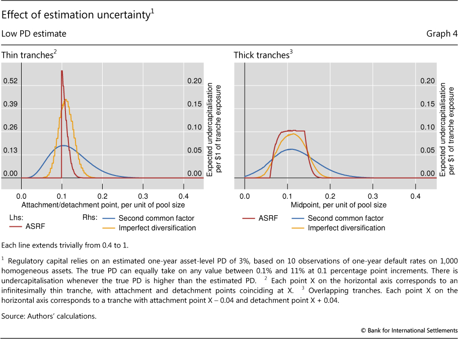
In the absence of regulatory safeguards for estimation error, there is a high likelihood of severe undercapitalisation of mezzanine tranches. We first show this in the context of an ASRF pool and for a PD estimate that is equal to 3%, which results in a pool-wide regulatory capital of $0.10 per $1 of exposure. The expected undercapitalisation across thin tranches from this pool is plotted by the red line in Graph 4 (left-hand panel). Tranches with detachment points below the pool-wide regulatory capital are fully capitalised, at $1 per $1 of exposure, and thus can never experience a capital shortfall. For tranches most vulnerable to the cliff effect - ie with attachment points slightly above the pool-wide regulatory capital - expected undercapitalisation is extremely high: $0.60 per $1 of exposure. Of course, expected undercapitalisation declines with the seniority of the thin tranche, ie as it becomes less likely that the true PD is sufficiently high to matter.
Expected undercapitalisation is also substantial in the other two pools (Graph 4, left-hand panel, blue and orange lines). As discussed earlier, residual risk in these pools' conditional losses weakens the cliff effect and results in regulatory capital being more evenly spread across tranches than in the ASRF pool (recall Graph 3, left-hand panel). As a result, capital shortfalls are also more evenly spread out. This is why expected undercapitalisation has a lower peak but affects a wider range of thin tranches.
In practice, attachment and detachment points differ, ie tranches are thick. As explained above, taking the PD estimate at face value leads to quite similar capital requirements for thick tranches across the three pool types (recall Graph 3, right-hand panel). Expected undercapitalisations are thus also similar: between $0.06 and $0.10 per $1 of exposure to mezzanine tranches with a thickness of 8 percentage points (Graph 4, right-hand panel).
To underscore the large magnitude of expected undercapitalisation for mezzanine tranches, we refer to vertical tranches from the same underlying asset pools. As such tranches are not subject to the cliff effect, the impact of estimation error on their regulatory capital is much smaller. Namely, the expected undercapitalisation is roughly $0.01 per $1 of exposure to a vertical tranche. If the pool were sliced into tranches of different seniority, this undercapitalisation would be concentrated in mezzanine tranches. This is shown by the area under any of the lines in the left-hand panel of Graph 4, which is also equal to $0.01.
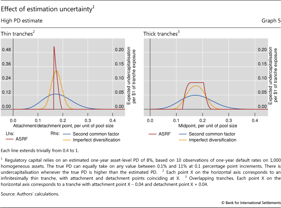
These results are robust to changes in the riskiness of the underlying portfolio. To gain intuition, note that an increase in the asset-level PD sets three forces in motion. First, all else the same, a higher asset-level PD is estimated with more noise, implying higher likelihood and severity of undercapitalisation. Second, in line with the regulatory model outlined in Annex 1, our setting accounts for an empirical regularity that a higher PD goes hand in hand with a lower default correlation.10 And the lower the default correlation, the lower the noise in PD estimates, all else the same.11 Third, regulatory capital is less sensitive to noise around high PD estimates than around low PD estimates (BCBS (2006), p 64). The second and third forces reduce the likelihood and severity of undercapitalisation and, in our stylised setting, roughly balance the effect of the first force.
A comparison between Graphs 4 and 5 - based on PD estimates of 3% and 8%, respectively - illustrates the weak dependence of tranches' expected undercapitalisation on the PD of the underlying assets. Indicating that a higher PD estimate translates into higher pool-level regulatory capital, the spike of the red line in the left-hand panel in Graph 5 occurs for a higher attachment/detachment point than the corresponding spike in Graph 4. Nevertheless the level of expected undercapitalisation - indicated by the heights of the lines - is remarkably similar across graphs.. This similarity remains for a wide range of PDs, including PDs as low as the regulatory target for banks, 0.1%.
Conclusion
Financial losses are uncertain. Banks and regulators rely on risk models to assess potential losses and set capital accordingly. However, not only are models simplifications of reality, but they also take as inputs parameters that are themselves estimated with uncertainty. The true value of a parameter can differ from the one that the bank or regulators based capital calculations on. This opens the door to uncertainty-driven undercapitalisation
We have shown in this article that the uncertainty inherent in estimating asset-level PDs will concentrate in mezzanine tranches and, if ignored, can lead to substantial undercapitalisation of these tranches. Our result is remarkable because it is obtained in the context of extremely simple and transparent asset pools, which should bring to a minimum the scope for estimation uncertainty. In other words, the result shows that the simplicity and transparency of the asset pool would not translate into simple-to-assess mezzanine tranches.
It is thus important to prevent the uncertainty inherent in risk assessments from raising the spectre of undercapitalisation and ultimately impairing the functioning of the securitisation market. Proposed changes to the regulatory framework for securitisations, which impose substantial capital safeguards on mezzanine tranches, would help avoid such an outcome (BCBS (2014)).
References
Bank for International Settlements (2008): 78th Annual Report, June.
Basel Committee on Banking Supervision (2006): Basel II: International convergence of capital measurement and capital standards: a revised framework - comprehensive version, June.
--- (2013): Revisions to the securitisation framework, consultative document, December.
Committee on the Global Financial System (2005): "The role of ratings in structured finance: issues and implications", CGFS Papers, no 23, January.
Duponcheele, G, W Perraudin and D Totouom-Tangho (2013): "A principles-based approach to regulatory capital for securitisations", Risk Control Working Paper.
European Banking Authority (2014): "EBA Discussion Paper on simple standard and transparent securitisations", EBA/DP/2014/02, October.
Fender, I and J Mitchell (2009): "The future of securitisation: how to align incentives", BIS Quarterly Review, September, pp 27-43.
Fender, I, N Tarashev and H Zhu (2008): "Credit fundamentals, ratings and value-at-risk: CDOs versus corporate exposures", BIS Quarterly Review, March, pp 87-101.
Gordy, M (2003): "A risk-factor model foundation for ratings-based bank capital rules", Journal of Financial Intermediation, vol 12, pp 199-232.
Hull, J and A White (2010): "The risk of tranches created from mortgages", Financial Analysts Journal, vol 66, no 5, pp 54-67.
--- (2012): "Ratings, mortgage securitizations, and the apparent creation of value", in A Blinder, A Lo and B Solow (eds), Rethinking the financial system, Chapter 7, Russell Sage Foundation.
Jones, D (2000): "Emerging problems with the Basel Capital Accord: regulatory capital arbitrage and related issues", Journal of Banking and Finance, no 24, pp 35-58.
Moody's Investors Service (2006): "Measuring corporate default rates", Special Comment, November.
Pykhtin, M and A Dev (2002): "Credit risk in asset securitisations: analytical model", Risk, vol 15(5), May, pp S16-S20.
Tarashev, N (2010): "Measuring portfolio credit risk correctly: why parameter uncertainty matters", Journal of Banking and Finance, no 34, September, pp 2065-76.
Annex 1: The ASRF model and securitisation tranches
Relying on the so-called Asymptotic Single Risk Factor (ASRF) model of credit losses (Gordy (2003)), the regulatory framework allows banks to calculate capital requirements at the level of individual exposures. Here, we outline the rationale behind such requirements when the exposure is to a securitisation or a securitisation tranche.
The ASRF model rests on two key assumptions. The first is that the bank's portfolio comprises infinitely many assets, each of negligible size. The second assumption is that a single common risk factor, Y, drives defaults. Concretely, focusing on asset i and denoting its idiosyncratic risk factor by Zi, the loss per unit of exposure to this asset, Li, is equal to:

In this expression, LGDi is loss-given-default, DPi is the default point, Ii indicates the default status, and the common factor loading ρi governs asset correlations. The benchmark horizon is one year.
A bank's regulatory capital is set equal to the highest level of portfolio losses that can be exceeded with a probability of 0.1%. Two key properties of the ASRF model facilitate the calculation of this level. First, all idiosyncratic risk is diversified away. This implies that the sum of asset-specific losses is a known decreasing function of the common risk factor: ∑i Li = f(Y). Then, denoting the 0.1 percentile of Y by y0.1, portfolio-wide regulatory capital is K = f(y0.1). Second, this capital can be allocated to individual assets, as it equals the sum of expected asset-level losses conditional on Y = y0.1: ie K = f(y0.1) = ∑i Ki = ∑i E(fi (y0.1)), where Ki = E(fi (y0.1)) is the asset-specific capital requirement.
To minimise the data burden on banks, the regulatory framework allows for further simplifying assumptions. Namely, it is assumed that the two risk factors affecting each asset are independent standard normal variables, that LGDi = 45% and that the common factor loading is a decreasing function of the corporate obligor's probability of default: ρi = ρ(PDi). The last assumption reflects the stylised fact that better creditworthiness rests on diversification on the obligor's side and, thus, on higher relative exposure to non-diversifiable, common risk factors. The upshot is that, abstracting from maturity adjustments, the only free parameters in the regulatory capital formula are the one-year probabilities of default of individual assets (BCBS (2006), p 64).
When an infinitesimally small exposure is a securitisation, the calculation of capital requirements involves two steps. First, denoting an asset in the securitised pool by j, the pool's overall regulatory capital is calculated as Kpool = ∑j E(fj(y0.1)). This sum is the expected pool-wide loss when the common risk factor is at its 0.1 percentile, ie when Y = y0.1. Second, Kpool is allocated across tranches of different seniority according to the associated expected loss when Y = y0.1. For the same attachment and detachment points of a tranche, this expected loss would change with the risk profile of the securitised pool.
Let the securitised pool itself satisfy the two key assumptions that the ASRF model requires from the bank's overall portfolio. In this case, conditional on Y = y0.1, pool-wide losses are known to be equal to Kpool. By construction, these conditional losses are sure to wipe out any tranche with a detachment point below Kpool. Thus, the regulatory capital per $1 exposure to such a tranche should be $1. Symmetrically, if the attachment point of a tranche is higher than Kpool, then this tranche is completely shielded from the pool's conditional losses and its regulatory capital should be $0.
Alternatively, let the pool still comprise a large number of small assets but allow for a second, pool-specific risk factor, Zpool. This is the setting in Pykhtin and Dev (2002), who assume that, for asset j in the securitised pool,  , where εj is an idiosyncratic shock. Duponcheele et al (2013) argue that a reasonable value for ρ* is 10%. Because of the pool-level uncertainty generated by Zpool, conditional on Y = y0.1, the expected loss on a tranche with a detachment point below Kpool will now be less than $1 per $1 exposure. And so will be the tranche's regulatory capital. Symmetrically, the regulatory capital will be above $0 for a tranche with an attachment point above Kpool.
Annex 2: Conditional probability of the true PD
In this Annex, we accomplish two tasks. First, we derive the probability distribution of the true probability of default PD* conditional on a particular estimate, . Second, on the basis of this distribution, we define expected undercapitalisation when regulatory capital is based on .
To compute the conditional distribution of PD*, Pr(PD*|), we need two pieces of information. The first is the prior distribution of PD*. To be unrestrictive, we assume that PD* can equally take on any of the values at 0.1 percentage point increments between 0.1% (which is the regulatory target for a bank PD) and 11% (which corresponds to a distressed entity). The second is the data-generating process, given by expression (A.1) in the previous Annex for PD = PD*, which delivers the empirical default rates used to derive . We assume that there are 10 one-year default rates each underpinned by 1,000 obligors.
Given these two pieces of information, the derivation of Pr(PD*|) involves four steps. First, the prior distribution of PD* provides directly the unconditional Pr(PD*). Second, given a PD*, Monte Carlo simulations of the available data deliver Pr(|PD*). Third, the weighted average of Pr(|PD*) across different values of PD*, using Pr(PD*) as weights, delivers the unconditional Pr(). Fourth, by Bayes' rule, Pr(PD*|) = Pr(|PD*) ∗ Pr(PD*)/Pr().
We can now compute the expected undercapitalisation of a securitisation tranche. Let the calculated capital for the tranche be K() and the desired capital be K(PD*). Then, expected undercapitalisation is the weighted sum of K(PD*)−K() across all values of PD* above , using Pr(PD*|) as weights.
1 The authors thank Magdalena Erdem for excellent research assistance, and Claudio Borio, Dietrich Domanski, Neil Esho, Marc Farag, Ingo Fender, Raquel Lago, Hyun Song Shin, Kostas Tsatsaronis and Christian Upper for useful comments. The views expressed are those of the authors and do not necessarily reflect those of the BIS.
2 For discussions of key drivers of the pre-crisis securitisation markets, see Jones (2000), CGFS (2005) and Hull and White (2012).
3 These proposals address various types of uncertainty, including model uncertainty, while our analysis focuses exclusively on estimation uncertainty.
4 The crisis revealed that certain banks were exposed both to tranches on their balance sheets and, through explicit or implicit guarantees, to tranches held by off-balance sheet conduits. This article does not address the distinction between on- and off-balance sheet exposures and assumes that a bank sheds an exposure through an outright sale to an unrelated entity.
5 For an extensive review of securitisation markets at the crisis outset, see BIS (2008), Chapter VI.
6 We choose this specific PD level in order to work with easy-to-read graphs. The article's takeaways remain unchanged in qualitative terms under more realistic, lower PDs.
7 As we abstract from uncertainty, our capital calculations do not incorporate the proposals in BCBS (2014).
8 For a different perspective on uncertainty in the realm of securitisations, see Fender and Mitchell (2009). They argue that, when a securitisation originator's uncertainty about tranche riskiness differs from that of an investor, the credibility of the securitisation process is at stake. To support this credibility, it is thus necessary to impose specific retention requirements on originators.
9 A discussion paper, EBA (2014), has published a list of proposed criteria that simple and transparent securitisations should satisfy. These criteria include: homogeneous underlying assets, well defined capital structures, enforceable repayment schedules and long performance history of the underlying assets.
10 A likely explanation of this regularity is that, in order to attain a low PD, obligors diversify away their exposure to idiosyncratic risks. But the flip side of reduced idiosyncratic risks is greater relative exposure to non-diversifiable, common risk factors. This means that the default of a low-PD obligor would tend to stem from a risk factor that is likely to adversely affect other obligors as well. Low-PD obligors would thus be more likely to default together than high-PD ones.
11 A higher default correlation implies that observed default rates are more likely to be either very large or very small, irrespective of the true underlying PD. Thus, the higher the default correlation, the less informative are the default rates and, ultimately, the noisier is the PD estimate.