How much income is used for debt payments? A new database for debt service ratios
Debt service ratios (DSRs) provide important information about the interactions between debt and the real economy, as they measure the amount of income used for interest payments and amortisations. Given this pivotal role, the BIS has started to produce and release aggregate DSRs for the total private non-financial sector for 32 countries from 1999 onwards. For the majority of countries, DSRs for the household and the non-financial corporate sectors are also available. This article explains the key concepts underlying the compilation of the new series and it shows that the DSRs are meaningful, even when derived from a relatively sparse set of aggregate data. A brief look at the evolution of DSRs in recent years highlights that they allow for a more comprehensive assessment of credit burdens than the credit-to-income ratio or simple measures of interest payments relative to income.1
JEL classification: C8, E50.
Debt forms a central part of the narrative of financial crises and financial cycles more generally. Leverage, often proxied at the aggregate level by the ratio of the stock of liabilities (ie debt) to income, has received much attention as an indicator of financial excesses and vulnerabilities. Less discussed, but equally important, is the debt service ratio (DSR), which captures the share of income used for interest payments and amortisations. These debt-related flows are a direct result of previous borrowing decisions and often move slowly as they depend on the duration and other terms of credit contracts. They have a direct impact on borrowers' budget constraints and thus affect spending.
Since the DSR captures the link between debt-related payments and spending, it is a crucial variable for understanding the interactions between debt and the real economy. For instance, during financial booms, increases in asset prices boost the value of collateral, making borrowing easier. But more debt means higher debt service ratios, especially if interest rates rise. This constrains spending, which offsets the boost from new lending, and the boom runs out of steam at some point. After a financial bust, it takes time for debt service ratios, and thus spending, to normalise even if interest rates fall, as principal still needs to be paid down. In fact, the evolution of debt service burdens can explain the dynamics of US spending in the aftermath of the Great Financial Crisis fairly well.2 In addition, DSRs are also highly reliable early warning indicators of systemic banking crises.3
Given this pivotal role, the BIS has started to produce and release aggregate DSRs for the total private non-financial sector on a regular basis.4 The new DSR database currently covers quarterly series for 32 countries from 1999 onwards. For the majority of countries, series for the household and the non-financial corporate (NFC) sectors are also available. To derive the DSR on an internationally consistent basis, we apply a unified methodological approach and use, as far as they are available, input data that are compiled on an internationally consistent basis.
The methodology, the data inputs and some results are discussed in the remainder of this article.
Methodology
The DSR is defined as the ratio of interest payments plus amortisations to income. As such, the DSR provides a flow-to- flow comparison - the flow of debt service payments divided by the flow of income.
At the individual level, it is straightforward to determine the DSR. Households and firms know the amount of interest they pay on all their outstanding debts, how much debt they have to amortise per period and how much income they earn. But even so, difficulties can arise. Many contracts can be rolled over so that the effective period for repaying a particular loan can be much longer than the contractual maturity of the specific contract. Equally, some contracts allow for early repayments so that households or firms can amortise ahead of schedule. Given this, deriving aggregate DSRs from individual-level data does not necessarily lead to good estimates.5 And such data are rarely comprehensive, if available at all. For this reason, we derive aggregate DSRs from aggregate data directly.
While interest payments and income are recorded in the national accounts, amortisation data are generally not available and hence present the main difficulty in deriving aggregate DSRs. To overcome this problem, we follow an approach used by the Federal Reserve Board to construct debt service ratios for the household sector (Dynan et al (2003)) which measures amortisations indirectly. It starts with the basic assumption that, for a given lending rate, debt service costs - interest payments and amortisations - on the aggregate debt stock are repaid in equal portions over the maturity of the loan (instalment loans). The justification for this assumption is that the differences between the repayment structures of individual loans will tend to cancel out in the aggregate.6 Using some simulations, we show in Box 1 that this indeed seems to be the case. For instance, approximating the aggregate DSR with the instalment loan formula works, though with a small approximation error, even if the majority of borrowers pay back the principal only at the end of the contract.
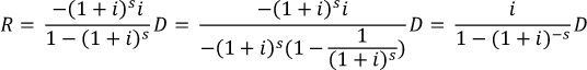
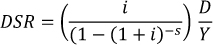
By using the standard formula for the per-period cost of an instalment loan (see Box 2 for a derivation) and dividing it by income, the aggregate DSR for sector j at time t can be calculated as:
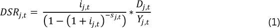
where Dj,t denotes the total stock of debt, Yj,t denotes aggregate income available for debt service payments, ij,t denotes the average interest rate on the existing stock of debt and sj,t denotes the average remaining maturity across the stock of debt. Given that the new database has a quarterly frequency, we match flows to flows on a quarterly basis. Thus, we use quarterly income and the average interest rate per quarter, and we measure the remaining maturities in quarters.
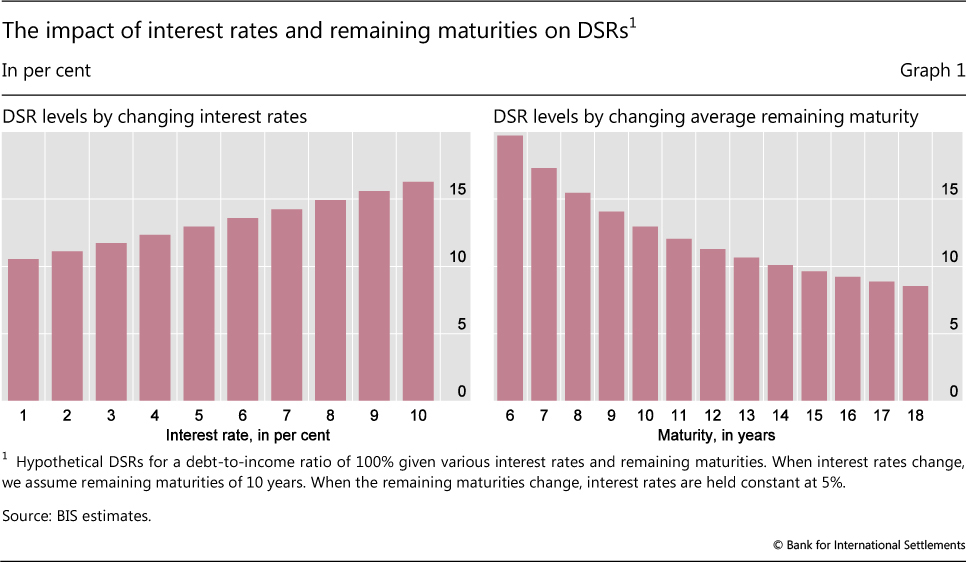
The instalment loan formula indirectly captures amortisations through the non-linear interest rate term in the denominator. To provide some understanding of how amortisations affect the DSR as interest rates and maturities change, consider a simple example with two sectors, each with a stock of debt of 100 and income of 100. In both sectors, the average remaining maturity of the debt stock is 10 years, but sector A has borrowed at an average interest rate of 2%, whilst sector B has an average interest rate of 5%. Given the interest rate differential, one would expect a substantially lower debt service ratio in sector A. This is not the case, however, because of amortisations. In fact, despite interest payments being 60% lower in sector A, its DSR is only slightly smaller: 11%, compared with 13% in sector B. Now consider a third sector, C, which is similar to sector B in that it also has a debt-to-income ratio of 100% and borrows at an average interest rate of 5%, but it faces an average remaining maturity of only six years. In this case, its DSR is close to 20% rather than 13%. These non-linear effects are illustrated further in Graph 1, which shows hypothetical DSRs for a debt-to-income ratio of 100% over a range of interest rates (Graph 1, left-hand panel) and remaining maturities (Graph 1, right-hand panel).
A potential concern with the instalment loan formula is that the non-linear effects from the "amortisations" term can generate an approximation error when aggregate data are used. For example, applying formula (1) to individual loans and summing up does not produce the same DSR which would be obtained from applying it to aggregate data inputs directly. Nevertheless, this approximation error turns out to be relatively independent of average interest rates, debt-to-income ratios or maturities (Box 1). Thus, our methodology should correctly capture how the DSR in a particular country changes over time, even if it does not necessarily accurately measure its level relative to what one could obtain from the correct micro data. The Fed encountered similar issues in relation to its household DSRs, pointing out that its "approximation is useful to the extent that, by using the same method and data series over time, it generates a time series that captures the important changes in the household debt service burden" (Federal Reserve Board (2013)).
Data inputs for constructing DSRs
The previous section has shown that it is possible to construct meaningful aggregate DSRs with a relatively sparse set of aggregate data: the total stock of debt, the income available for debt service payments, the average interest rate on the existing stock of debt and the average remaining maturity. This is encouraging and simplifies our task considerably because it lessens the need for micro-level data, which are not available for a large range of countries and time periods.
This section provides a high-level overview of the data inputs. Further details and country-specific information are provided in the data documentation.7 To ensure international consistency, we rely as much as possible on data from national accounts. In particular, national accounts provide us with information about the stock of debt, income and interest rates.8
We measure the stock of debt for each sector by its credit counterpart as recorded in the BIS database on credit to the private non- financial sector (Dembiermont et al (2013)).
To capture the income available to service the debts of households or non-financial corporations (NFCs), we augment gross disposable income (GDI) with gross interest payments, as GDI measures income after such payments. In the case of NFCs, we also add dividends, as these are discretionary and could be reduced if debt service payments become too large. The sum of the two comprises the income of the total private non-financial sector.9
To accurately measure aggregate DSRs, the interest rate has to reflect average interest rate conditions on the stock of debt, which contains a mix of new and old loans with different fixed and floating nominal interest rates attached to them.
The average interest rate on the stock of debt is computed by dividing gross interest payments plus financial intermediation services indirectly measured (FISIM) by the stock of debt. FISIM is an estimate of the value of financial intermediation services provided by financial institutions. When national account compilers derive the sectoral accounts, parts of interest payments are reclassified as payments for services and allocated as output of the financial intermediation sector. In turn, this output is recorded as consumption by households and NFCs. As we are interested in the total burden of interest payments on borrowers regardless of their economic function, we add FISIM back to the interest payments reported in the national accounts.10
The average interest rate derived from national accounts is closely aligned with the lending rate on the stock of credit on banks' balance sheets (Graph 2, left-hand panel). Differences exist because the national account data capture a broader range of debt instruments than do the banking data. But the close alignment of both rates suggests that similar DSR estimates are obtained regardless of which rate is used. Hence, banking sector lending rates can be used as a proxy in cases where national account data are not available.11
Estimating average remaining maturities is difficult, as the data are usually not available. Some sources provide information on contractual maturities. But these may differ from actual maturities - for instance, because of rollovers and other forms of refinancing.12 And, as discussed, we are mainly interested in actual maturities because they determine the amount of money households and firms have to dedicate to amortising debt. We therefore have to rely on judgment, backed by as much evidence as is available. As we will show, potential mistakes mainly lead to a shift in the level of estimated DSRs, but will not affect their dynamics over time.
Box 1
Does using aggregate information to construct aggregate DSRs introduce distortions?
This box analyses how sensitive our approach is to aggregation assumptions. We start by showing that aggregate amortisation can indeed be estimated by assuming that the outstanding stock of debt is repaid in equal instalments, even though credit contracts are structured in a multitude of fashions at the micro level. Since the instalment loan formula is non-linear, however, the use of aggregates for the interest rate, the average remaining maturity, the debt stock and income will distort the picture relative to what one might obtain if one had access to more granular data. We show in this box that this distortion is relatively constant even when underlying inputs change. This indicates that our approach may lead to a potential misestimation of the level of the DSR, but generally have little influence on dynamics.
To assess potential aggregation effects, we simulate a debt stock consisting of 1,000 artificial loans that differ in size, interest rate, average remaining maturity and income of the borrower. All input variables are random. In the base case, debt-to-income ratios average 150%, interest rates 5% and average remaining maturities 15 years. The distributions of these variables across loans are calibrated in such a way that the resultant distribution of individual debt service ratios in the base case is very similar to the distribution of household debt service ratios in Canada and the United States.
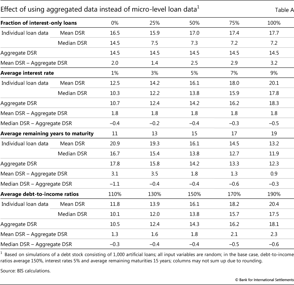
The simulation highlights that, while our methodology produces an approximation error, this is little related to the instalment loan assumption. To check the validity of this assumption, we let the fraction of instalment loans vary between zero and 100%. The remaining loans in this case are interest-only loans, of which only 1/15 involve repaying the principal in each period, in line with an assumption that the average remaining maturity is 15 years. The upper panel of Table A shows the difference between using micro data and relying on aggregate data plus the instalment loan formula. On average, the two approaches differ by around 2.5 percentage points. But this difference varies only between 1.4 and 3.2 percentage points depending on our assumption about the share of interest-only loans.
 This variation is small, especially given that the composition of the loan portfolio is unlikely to change to such a degree within a particular country. As such, it indicates that the instalment loan assumption works well for constructing aggregate DSRs.
As discussed in the main text, while the main source of approximation error arises from the use of aggregate information, this more likely distorts the estimated mean of the DSR than its dynamics. In particular, the size and direction of this error remain fairly constant, as the overall levels of interest rates, debt-to-income ratios or maturities change. In the base case (average debt-to-income ratio = 150%, average interest rate = 5% and average remaining maturity = 15 years), the average DSR of the individual loans is 16.1%, which is 1.9 percentage points higher than the estimated DSR of 14.2%. If interest rates on average increase to 9%, the average DSR of individual loans rises to 20.1% and the estimated DSR rises to 18.3%, but the estimation error remains approximately the same, at 1.8 percentage points. Similar results emerge for changes in the average remaining maturity or debt-to-income ratios. Interestingly, the approximation error is even lower if we compare the estimated DSR with the median of the individual data. In any case, note that the ranges of the input parameters in this simulation are rather large. For instance, we simulate debt-to-income ratios from 110% to 190%, but it took around 20 years for the debt-to-income ratio for the total private sector in the United States to increase from 110% to 150%. Similarly, an increase in the average remaining maturity from 15 to 19 years (we simulate remaining maturities between 11 and 19 years) would require a doubling of the average remaining maturity on more than 25% of the outstanding loans, which is not likely to happen. The characteristics of the loan stock are thus likely to be relatively stable over time. This argues for the accuracy of the aggregate approach for estimating DSRs.
Based on the Consumer Expenditure Survey, Johnson and Li (2010) report the following distribution of household debt service burdens in the United States from 1992 to 2004: 6% (20th percentile), 12% (40th percentile), 19% (60th percentile) and 28% (80th percentile). Calculating debt service burdens based on an instalment loan formula, the corresponding values in our sample are 2% (20th percentile), 10% (40th percentile), 17% (40th percentile) and 27% (80th percentile). The simulated distribution also broadly matches the distribution and main statistics of household DSRs in Canada from 1999 to 2000 (Faruqui (2008)). When checking the instalment loan assumption, we increased the sample size to 30,000, to avoid small- sample problems, when the fraction of interest-only loans that repay the principal is low. The median drops rapidly with the fraction of interest-only loans by construction, as 14/15 of the interest-only loans are not amortised at all.
For the household sector, we apply a constant 18-year average remaining maturity across countries and time. Two different approaches lead to this assumption. First, 18 years emerges as the average across countries, if we assume an average remaining maturity of 20 years for mortgages13 and six years for consumer loans,14 and weight these values by the respective share in households' total debt (Graph 2, centre panel). Alternatively, for some countries, we have information on the amount of household loans on banks' balance sheets grouped into three broad buckets of initial contractual maturities.15 Taking a weighted average across maturity buckets leads again to an average remaining maturity for household loans of around 18 years in all countries (Graph 2, centre panel). Interestingly, in both cases the variation across countries is small, supporting the use of a constant average maturity across countries. This simplifies the approach, and in any event using country-specific remaining maturities that vary from 16 to 19 years would not alter the DSRs significantly.
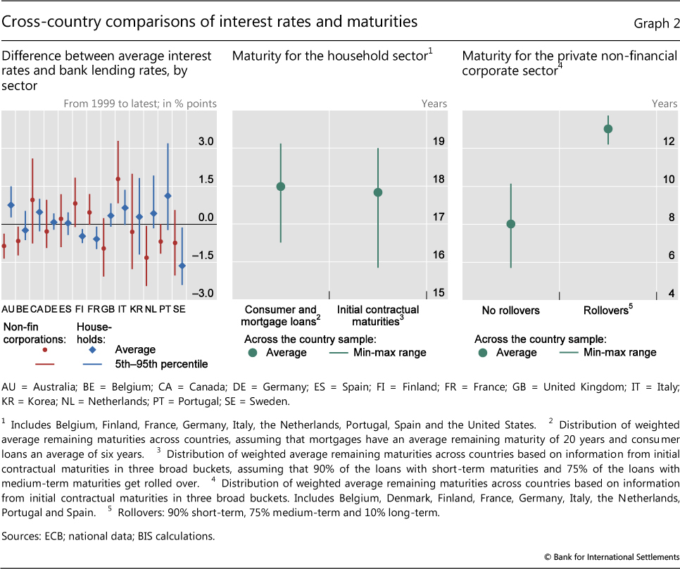
For the non-financial corporate sector, we apply a 13-year average remaining maturity. This value is more judgmental than in the case of the household sector, because we have little information on actual amortisations. However, we know that refinancing to extend maturity is very important. For instance, around 45% of bonds or syndicated loans are refinanced (Mian and Santos (2011), Xu (2015)).16 Applying this rollover assumption leads to a substantially higher estimate of the average remaining maturity than is evident from contractual maturities (Graph 2, right-hand panel).17 It also makes the estimates more similar across both time and countries, despite large changes in contractual maturities in some countries. For example, in Spain, 40% of the loans had a contractual maturity of less than one year in the late 1990s, whereas only 20% do now.
For the total private non-financial sector, we assume that the maturity is a weighted average of the maturities in the two subsectors. The weights are given by the share of debt in each sector compared with the total amount of private non-financial debt.
Box 2
Derivation of the DSR formula
In this box, we derive the instalment loan formula. We also show how we derive remaining maturities from contractual maturities.
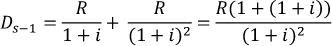
To understand the instalment loan formula, consider a loan of size D with a per-period interest rate of i and a maturity of s periods. Let Dt denote the remaining principal in period t, with D=D1. Suppose that the per-period debt costs, Rt, are paid in equal portions over the maturity of the loan, ie R=R2=-=Rs, which means that the loan is structured as a so called instalment loan. How large is the debt cost, R, given D, i and s?
To derive a formula for R, consider what we know about debt costs in each period. In the first period, for instance, the payment must satisfy R=iD+D-D2 and in the t:th period R=iDt+Dt-D(t+1). In the last period, s, the payment satisfies iDs+Ds-D(s+1) , but since there is no remaining principal in period s+1, ie D(s+1) =0, we have:

This expression can then be used to derive the payment in the second-to-last payment period, which gives:
Continuing recursively in this fashion until the first payment period, we get:
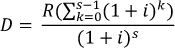
which, using the formula for a finite geometric sum, becomes:
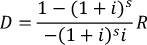
Solving for R gives:
Defining the debt service ratio as DSR=R/Y, where Y denotes income, we have the desired formula:
Given that borrowers can roll over debt with some probability, how can we estimate maturities from information on initial contractual maturities? Consider a portfolio of loans with a contractual maturity of c periods. At maturity, each loan has a probability ρ of getting renewed for another c periods. Then, the maturity, s, of the portfolio satisfies:


and using the formula for the infinite sum of an arithmetico-geometric sequence gives:
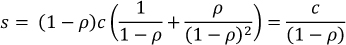
Hence, the remaining contractual maturity can be simply calculated by dividing the contractual maturity by one minus the rollover probability.
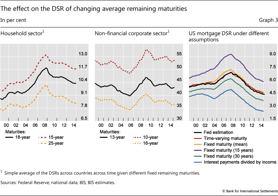
Even if our estimates for remaining maturities are inaccurate, this will mainly affect the level rather than the dynamics of DSRs. The solid lines in the left-hand and centre panels of Graph 3 show the average sectoral DSRs across countries, using the baseline assumption of 18 and 13 years for the household sector and the non-financial corporate sector, respectively. The dotted lines show DSRs under alternative maturity assumptions. As can be seen from the graph, changes in the assumptions about remaining maturities have a first-order impact on the level but not on the dynamics of the estimated DSRs for both sectors. When we apply a higher maturity, the DSR naturally moves down since the loans are amortised over a longer period of time, while the opposite is true for lower maturities.
Keeping remaining maturities fixed across time and across countries is appealing because of its simplicity, but it may distort our estimates somewhat, beyond shifts in the level. Yet, as long as the structure does not change significantly and permanently, deviations are likely to be small and temporary. This can be illustrated for the US mortgage sector, where we have information on actual remaining maturities and the Federal Reserve's own estimate of the mortgage debt service ratio as a reference point. Using time-varying average remaining maturities allows us to replicate the Fed's estimates (black and red lines, right-hand panel of Graph 3).18 If we hold remaining maturities constant at their historical mean instead (yellow line), we overestimate the increase in the mortgage DSR around the financial crisis, as in fact average remaining maturities in that period rose from 21 to 24 years and then fell back. However, despite a substantial shift in remaining maturities, the difference between the DSRs based on time-varying and constant maturities is less than half a percentage point at any given point.19 The level shift from applying "wrong" remaining maturities is clearly visible in the graph. For instance, the dynamics of the debt service ratio are essentially unaffected whether we assume a remaining maturity of 15 years (purple line) or 30 years (green line).
The US example highlights again that it is important to take amortisations into account when assessing debt-related payments for households and firms. Mortgage interest payments alone relative to income (blue line) looked sustainable compared with historical levels, even at the height of the crisis.20 But once one accounts for amortisation, debt service ratios were substantially higher than in earlier periods or several years after the crisis.
The evolution of DSRs over the last 15 years
In this section, we use the BIS estimates to study the evolution of the DSR in different countries over the last 15 years. Given the difficulties in pinpointing the level accurately, it is more meaningful to compare national DSRs relative to their means rather than comparing their absolute levels. In a cross-country context, such an approach will also take care of different institutional and behavioural factors affecting average remaining maturities. In particular, it is unlikely that the 18- and 13-year assumed maturities for the household sector and the non-financial corporate sector, respectively, will be fully accurate for all countries. Given that, as already discussed, average remaining maturities mainly affect the level and not the dynamics of the DSR, removing cross-country specific means allows for a more appropriate cross-country comparison of how DSRs have evolved over time.
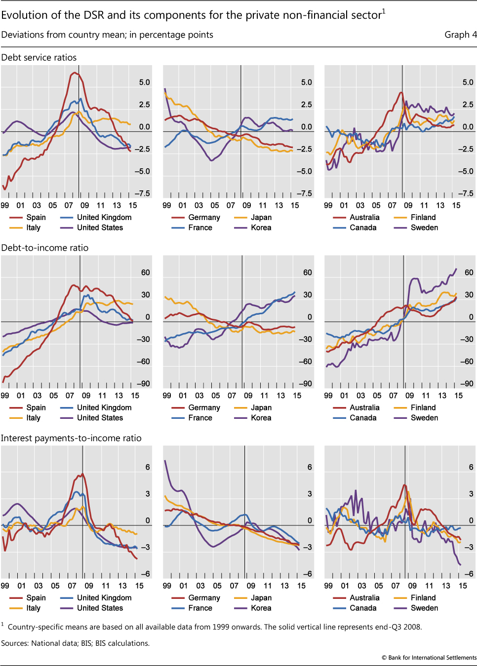
Graph 4 illustrates how the DSR provides a more comprehensive assessment of debt burdens than the debt-to-income ratio or simple measures of interest payments relative to income, because it takes both interest payments and amortisations into account. This is clearly visible in the case of France or Korea. Debt-to-income ratios have been rising in both countries since the early 2000s (Graph 4, centre panels). At the same time, interest rates - and with them interest payments-to-income ratios - have followed a downward trend (Graph 4, bottom panels), allowing households and firms to carry larger amounts of debt with the same amount of income. In the case of Korea, the DSR for the total private non- financial sector has been fluctuating around a broadly stable trend. For France, on the other hand, the increase in debt-to-income ratios has outweighed the fall in interest rates, leading to an overall rise in the DSR (Graph 4, top centre panel).
As such, DSRs provide an explanation for the limited amount of deleveraging that has taken place since the financial crisis, as documented by Buttiglione et al (2015), among others. Whereas debt-to-income ratios have been slow to fall, DSRs have dropped substantially in countries such as Spain, the United Kingdom and the United States (Graph 4, top left-hand panel), mainly due to the reduction in interest rates. Nonetheless, debt service ratios took several years to return to normal levels, helping to explain the weak post-crisis recovery (Juselius and Drehmann (2015)). DSRs are now below their sample average in many countries. Together with exceptionally low interest rates, this may reduce the incentives for further deleveraging.
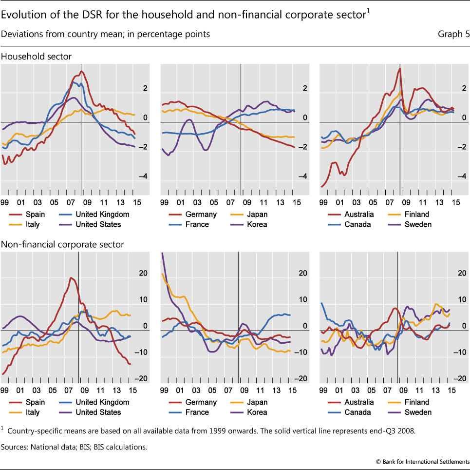
DSRs can also provide a gauge of the sustainability of credit developments. For example, in Spain, the United Kingdom and the United States, household DSRs increased substantially ahead of the financial crisis (Graph 5, top left-hand panel). In Spain and the United Kingdom, this was accompanied by growing non-financial corporate DSRs (Graph 5, bottom left-hand panel). These developments are typical ahead of financial crisis. Indeed a rapid rise in DSRs has been found empirically to be a strong early warning indicator of systemic banking crises (Drehmann and Juselius (2014)).
At present, DSRs point to lower debt service burdens in some countries and sectors, but a substantial increase in others. For instance, non- financial corporate sector DSRs have been rising in Finland and Sweden, reaching high levels in comparison with cross-country benchmarks (Graph 5, bottom right-hand panel).
Conclusion
This special feature provides an introduction to the new BIS database on aggregate debt service ratios. The database currently covers DSRs for the total private non-financial sector for 32 countries, as well as DSRs for the household and the non- financial corporate sectors separately for 17 countries.
From a methodological perspective, the main contribution of the article is to show that it is possible to construct consistent and meaningful DSRs for a large set of countries with a relatively sparse set of aggregate data. Whilst the use of more granular data may result in different estimates for DSR levels, our methodology captures the dynamics of DSRs over time quite well. For practical purposes, the difficulties in pinpointing the DSR level imply that it is most meaningful to compare our estimates of the DSR over time, and to remove country-specific means.
Looking forward, efforts are under way to increase the time and country coverage of the database. This will allow users a broader historical and global perspective, which is important given the pivotal role of debt service burdens as a link between business and financial cycles.
References
Alessi, L, A Antunes, J Babecký, S Baltussen, M Behn, D Bonfim and D Zigraiová (2014): "Comparing different early warning systems: results from a horse race competition among members of the macro-prudential research network", paper presented at the final conference of the Macroprudential Research Network.
Buttiglione, L, P Lane, L Reichlin and V Reinhart (2014): "Deleveraging? What deleveraging?", Geneva Reports on the World Economy.
Dembiermont, C, M Drehmann and S Muksakunratana (2013): "How much does the private sector really borrow - a new database for total credit to the private non-financial sector", BIS Quarterly Review, March, pp 65-81.
Drehmann, M and M Juselius (2012): "Do debt service costs affect macroeconomic and financial stability?", BIS Quarterly Review, September, pp 21- 34.
--- (2014): "Evaluating early warning indicators of banking crises: satisfying policy requirements", International Journal of Forecasting, vol 30(3), pp 759- 80.
Dynan, K, K Johnson and K Pence (2003): "Recent changes to a measure of US household debt service", Federal Reserve Bulletin, vol 89(10), pp 417-26.
Faruqui, U (2008): "Indebtedness and the household financial health: an examination of the Canadian debt service ratio distribution", Bank of Canada, Working Papers, no 46, December.
Federal Reserve Board (2013): "Household debt service and financial obligations ratios. About the release", December.
Johnson, K and G Li (2010): "The debt-payment-to-income ratio as an indicator of borrowing constraints: evidence from two household surveys", Journal of Money, Credit, and Banking, vol 42(7), pp 1373-90.
Juselius, M and M Drehmann (2015): "Leverage dynamics and the real burden of debt", BIS Working Papers, no 501, May.
Mian, A and J Santos (2011): "Liquidity risk, maturity management and the business cycle", mimeo.
Xu, Q (2015): "Kicking maturity down the road: early refinancing and maturity management in the corporate bond market", University of Chicago Booth School of Business, job market paper.
1 We would like to thank Christian Dembiermont, whose statistical knowledge was invaluable for the compilation of the series. We are also grateful for input from national central banks. This article benefited from useful comments by Claudio Borio, Ben Cohen, Dietrich Domanski, Hyun Song Shin and Suresh Sundaresan. The views expressed in it are those of the authors and do not necessarily reflect those of the BIS.
2 See Juselius and Drehmann (2015) for a formal analysis.
3 See Alessi et al (2014) or Drehmann and Juselius (2014).
4 The series are available on the BIS website at www.bis.org/statistics/dsr.htm.
5 Consider an example of a household that buys a house and borrows CHF 500,000. The initial mortgage contract runs over 10 years. But the loan is structured on the premise that the borrower can refinance it after 10 years and that he will pay it back in full over a 25-year period. It then makes sense to estimate the DSR under the assumption that the loan has a 25-year maturity. But this may not be known when constructing aggregate DSRs from micro data. In addition, recorded repayment flows may not reflect actual amortisations. For example, after 10 years the household changes its mortgage provider, repaying the original bank CHF 320,000 in year 10, but financing CHF 300,000 of this amount with a new loan from a different bank. Micro-level data might record a repayment of CHF 320,000, even though the repayment by the household is CHF 20,000.
6 This aggregation assumption is also intuitive. For example, consider 10 loans of equal size for which the entire interest payment and principal are due at maturity, each with 10 repayment periods and taken out in successive years over a decade. After 10 periods, when the first loan falls due, the flow of interest payments and amortisations on these 10 loans will jointly be indistinguishable from the repayment of a single large instalment loan.
7 See www.bis.org/statistics/dsr.htm.
8 For 15 countries in the sample, only the DSR for the total private non-financial sector (PNFS) is currently available given data availability. In these cases, income is proxied by nominal quarterly GDP series and the interest rate is proxied by the average interest rate on loans made by banks to the PNFS.
9 This is the best approximation for the income of the PNFS which correctly matches the definition and scope of the credit series. There is a degree of double- counting, though, as some dividends from the NFCs are paid to households. However, the amount concerned is very small and does not have a significant impact on the income measure and hence on the final DSR.
10 The FISIM component relative to total interest payments can vary across time. For the household sector in our sample, it is, for instance, estimated to be about 30% on average.
11 For a few countries, even average lending rates on the stock of bank debt are not available. Instead, we use the short-term money market rate plus the average markup between lending rates and the money market rates across countries, as this provides a reasonable approximation (Drehmann and Juselius (2012)).
12 From a financial stability perspective, it can also be useful to look at debt service burdens that take contractual remaining maturities into account. The shorter they are, the higher the rollover risks and potential disruptions to economic activity if banks are not willing to refinance maturing loans.
13 Mortgages are typically repaid over 25-30 years in advanced countries. In the simplest case, where the volume of loans taken out over consecutive years is always the same, the credit-weighted average remaining maturity across new and old (partially repaid) loans is between 16 and 19 years. If new borrowers take out larger nominal loans than old ones, which historically has happened, for instance, because of rising house prices, the weighted average remaining maturity of the stock of credit is higher, suggesting a figure of about 20 years. This is closely in line with the average remaining maturity of 21 years in the United States that has prevailed since the early 1990s, as shown by the biannual American Housing Survey (see http://www.census.gov/programs-surveys/ahs/data.html).
14 An average remaining maturity of six years for consumer loans provides the best fit when trying to replicate the Fed's DSR for consumer loans. This is also consistent with the weighted average remaining maturity of 6.5 years for consumer loans in the United States that has prevailed since 1980.
15 The three buckets are loans with initial contractual maturities of less than one year, between one and five years and above five years. We then assume that these buckets correspond to remaining maturities of one, three and 20 years, respectively. We also assume that 90% of the loans with short maturities and 75% of the loans in the middle bucket get rolled over (Box 2 discusses how rollovers affect remaining maturities). Dropping the rollover assumption shortens the average remaining maturities to 17.2 years and increases the cross-country variation somewhat.
16 Mian and Santos (2011) show that the refinancing probability varies with the business cycle, ranging from 45% in downturns to about 60% in booms. We choose the lowest value for two reasons. First, using the lower value gives DSR estimates that better capture incipient debt servicing constraints during booms. Second, not all refinances are extended with the same maturity as in the original loan, whereas we assume this to be the case.
17 Similarly to the household sector, we use banks' balance sheet data on non-financial corporate sector loans divided into three buckets according to whether the initial contractual maturities are less than one year (short-term loans), one to five years (medium-term loans) or above five years (long-term loans). For each bucket, we take the average maturity from data on the initial maturities of all corporate bonds from 1990 to the present for advanced economies available in Dealogic. This gives us average initial maturities of 0.92, 3.5 and 13.3 years for the three buckets, respectively. As short-term loans are rolled over more frequently than long-term ones, we assume that 90% of short-term loans, 75% of medium-term loans and 10% of long-term loans are refinanced, in order to match the average refinancing probability of 45% suggested by the literature.
18 When constructing this estimate, we follow the Fed and assume a minimum repayment of 2% in each quarter for revolving consumer loans (ie 98% can be rolled over) and an average remaining maturity of other consumer loans of four years, in line with initial contractual maturities of five to six years, as observed for cars or student loans in the United States.
19 Given the inherent non-linearity in the instalment loan formula, a three-year shift in aggregate remaining maturities - for example, from 10 to 13 years - would have had a proportionally bigger impact.
20 Note that, while relatively small changes in the assumption about remaining maturity do not meaningfully affect the overall trend, extreme maturity assumptions would matter: for example, assuming a remaining maturity of 100 years would be misleading, as repayments in this case would be so low that the DSR and the ratio of interest payments to income would coincide.