Evaluating EWIs with the AUC
(Extract from pages 60-61 of BIS Quarterly Review, March 2014)
The AUC (the area under the receiver operating characteristics curve, or ROC curve) is a statistical tool used in assessing the performance of signals that forecast binary events (ie events that either occur or do not). The term ROC reflects the origins of the tool in the analysis of radar signals during World War II, although it has a long tradition in other sciences (eg Swets and Picket (1982)). Its applications to economics are more recent (eg Cohen et al (2009), Berge and Jorda (2011), Jorda et al (2011)). The AUC summarises the trade-off between correct and false signals for all different operator (policymaker) preferences, as explained below.
Selecting an indicator involves making a choice on the trade-off it offers between the rate of correct event predictions and the rate of false calls. There are four possible value combinations of a binary signal (which can be "on" or "off") and subsequent event realisations ("occurrence" or "non-occurrence"). The perfect indicator signals "on" ahead and only ahead of all occurrences, while the signal from an uninformative indicator has an equal probability of being right or wrong. Signals from continuous variables (such as those considered in this article) must be calibrated. This means that the operator will define a threshold and consider as a signal a value of the indicator variable that exceeds this threshold. Varying the threshold varies the relationship between true positives (signal "on" and "event occurs") and false positives (signal "on" and "non-occurrence"). If it is set at a very high value, the indicator will miss many events but it will also make very few false positive signals. A very low threshold value will generate many signals, capturing more events but also making many more false calls.
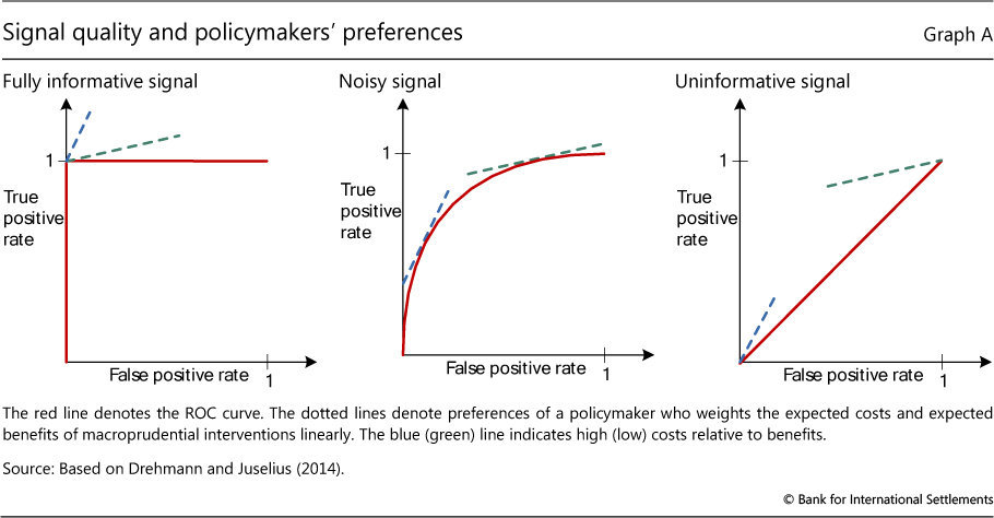
The ROC curve for an indicator captures the relationship between the rate of true positives (as a share of all occurrences) and the rate of false positives (as a share of all non-occurrences) for different values of the threshold. The red lines in the graph below illustrate the ROC curve for three different indicators. The left-hand panel corresponds to the perfect indicator. Since the indicator is able to perfectly signal occurrences, decreasing the threshold value from the maximum implies that more and more events are predicted without any false calls being made (vertical segment). When the threshold is set so as to capture all occurrences, lowering it further will not increase the rate of correct predictions, which is already at 1, but will add to the rate of false calls (horizontal segment). The right-hand panel shows the other extreme: the completely uninformative indicator. Lowering the threshold in this case changes the true positive and false positive rates, but always by the same amount. The trade-off is thus depicted by the 45° line. The more interesting cases are between the extremes (centre panel): as calibration moves away from the origin of the graph (by lowering the threshold from its maximum value), it initially improves the true positive rate at a low cost in terms of increases in the false positive rate. The cost of improving the true positive rate, however, increases (the ROC curve flattens) as the threshold is progressively lowered.
The operator (the policymaker) is not indifferent about this trade-off and assigns a positive weight to the success rate (correct predictions of occurrences) and a negative weight to the rate of false positives. These preferences are shown as straight lines. The steeper (blue dotted) line corresponds to an operator who dislikes false positives relatively more than another operator who is more interested in not missing an occurrence (green dotted line). Each operator tries to achieve the highest extension of the slope that represents their preferences. For the two extreme cases, the choice is trivial. In the case of the fully informative indicator, all operators will select the calibration that offers perfect accuracy. In the case of the uninformative indicator, the two operators will position themselves at opposite ends: one at the point of zero false positives and zero success rate (the origin), and the other at the point where all occurrences are captured but also the false positive rate is 100%. In realistic situations of informative but noisy indicators, each operator will select a different calibration as seen by the points of tangency in the centre panel. For each operator, the distance between the red line at the point of tangency and the 45° line represents the gain they obtain given their preferences and the options offered by the specific indicator.
The AUC is calculated as the area under the entire ROC curve. Intuitively, it captures the average gain over the uninformed case across all possible preferences of the operator (ie for all possible combinations of weights assigned to the two types of error). As such, it provides a summary measure of the signalling quality over the full range of possible preferences and calibrations (Elliott and Lieli (2013)). This is particularly appealing given the difficulties of offering precise quantification of the costs and benefits of macroprudential policymaking (CGFS (2012)). The uninformative indicator has an AUC equal to 0.5 (area under the 45° line), while that for the fully informative indicator is equal to 1. The intermediate cases have values in between. For indicators that decline ahead of events, the AUC takes values between 0.5 (uninformative) and zero (fully informative).
This assumes that the indicator increases ahead of an event. If the opposite is true, then a signal is "on" when the variable is below the threshold and the explanation is reversed.